Project Data, Structure & Paths

Project Management

Project Aims & Objectives

Tip

Before we begin, let’s clarify the aims of the project and learning objectives rest of the workshop.

Project Aim

We’ll be working with a subset of data from the NEON Woody plant vegetation survey. The aim of the project is to combine multiple files into a single analytical dataset and explore the data through visualisation and basic analysis.

Project Objectives

The nature of the data, which is spread across multiple files and tables with a lot of extraneous information, provides us a more realistic opportunity to practice what 50-80% of data analysis and modeling work actually is: data cleaning, combining and munging! From our raw data, the aim is to produce a clean analytical dataset using a reproducible R script.
Once we’ve produced our analytical data, we’ll move on to explore our data through visualisation using ggplot2 and perform some very basic analysis.
We’ll finally bring it all together, code, narrative, data and plots in scientific report generation with Quarto.

Project Data

We’re in our new project so the first thing we need to do is get the data we’ll be working with. This is a common start to any project where you start with a few data files. These might be generated through your own data collection, given to you by others or published data products and you might need to clean, wrangle and combine them together to perform your analysis.

Q: Where should I save my raw data files?

conventions: Data management

Store raw data in data-raw/: raw inputs to any pre-processing, read only.

Keep any processing scripts in the same folder
Whether and where you publish data depends on size and copyright considerations.

Store analytical data in data/: any clean, processed data that is used as the input to the analysis.

Should be published along side analysis.

Setting up a `data-raw/` directory

We start by creating a data-raw directory in the root of our project. We can use usethis function usethis::use_data_raw(). This creates the data-raw directory and an .R script within where we can save code that turns raw data into analytical data in the data/ folder.

We can supply a name for the analytical dataset we’ll be creating in our script which automatically names the .R script for easy provenance tracking. In this case, we’ll be calling it individual.csv so let’s use "individual" for our name.

usethis::use_data_raw(name = "individual")

✔ Setting active project to '/cloud/project'
✔ Creating 'data-raw/'
✔ Adding '^data-raw$' to '.Rbuildignore'
✔ Writing 'data-raw/individual.R'
• Modify 'data-raw/individual.R'
• Finish the data preparation script in 'data-raw/individual.R'
• Use `usethis::use_data()` to add prepared data to package

The data-raw/individual.R script created contains:

## code to prepare `individual` dataset goes here

usethis::use_data(individual, overwrite = TRUE)

We will use this file to perform the necessary preprocessing on our raw data.

However, in the mean time we will also be experimenting with code and copying code over to our individual.R script when we are happy with it. so let’s create a new R script to work in.

File > New File > R script

Let’s save this file in a new folder called attic/ and save it as file development.R.

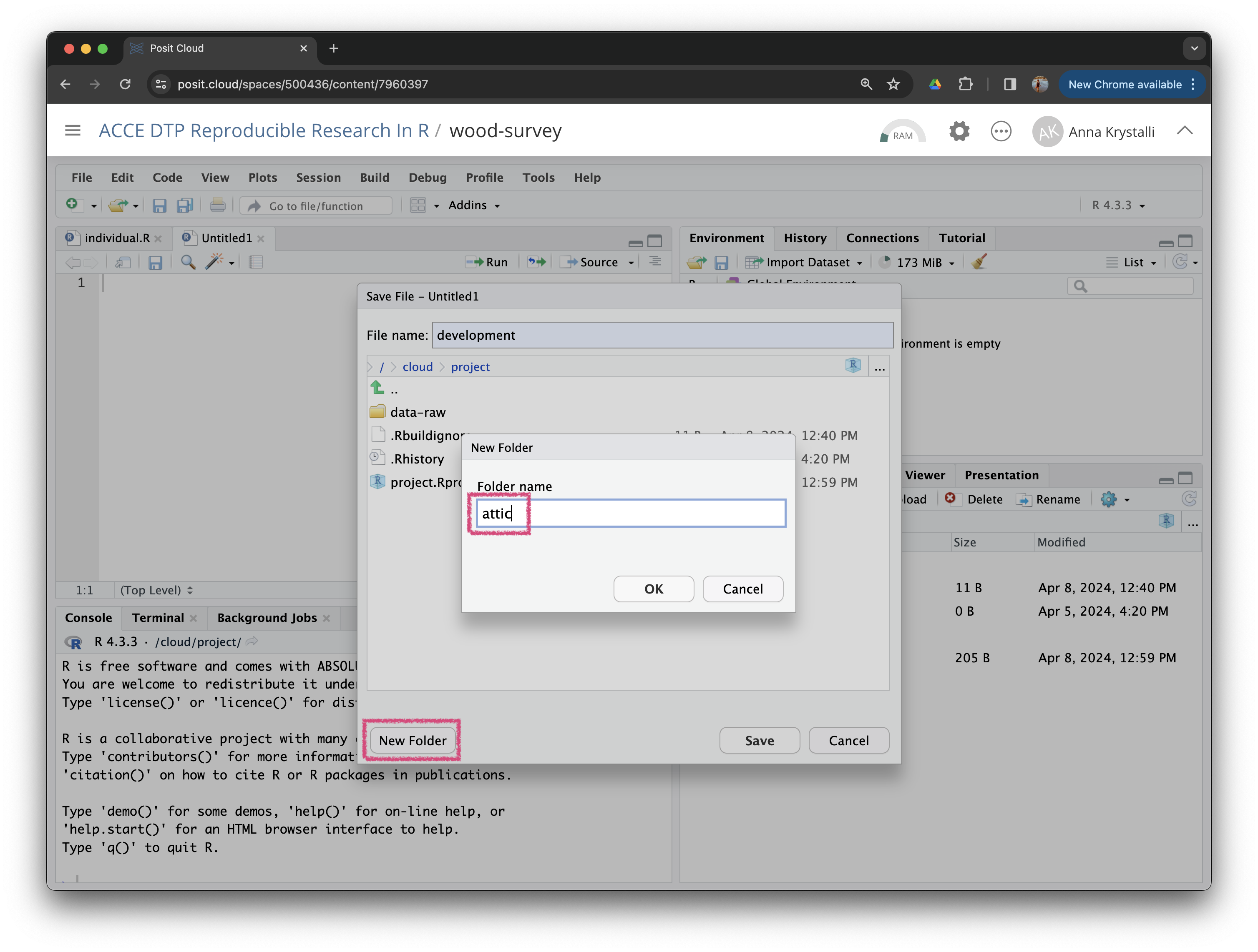
Let’s work in development.R for now.

Download data

Now that we’ve got our data-raw folder, let’s download our data into it using function usethis::use_course() and supplying it with the url to the materials repository (bit.ly/wood-survey-data) and the path to the directory we want the materials saved into ("data-raw").

usethis::use_course("bit.ly/wood-survey-data",
           destdir = "data-raw")

✔ Downloading from 'https://bit.ly/wood-survey-data'
Downloaded: 7.61 MB  
✔ Download stored in 'data-raw/wood-survey-data-master.zip'
✔ Unpacking ZIP file into 'wood-survey-data-master/' (77 files extracted)
Shall we delete the ZIP file ('wood-survey-data-master.zip')?

1: Nope
2: No way
3: I agree

Selection: 3
✔ Deleting 'wood-survey-data-master.zip'

NEON Data

The downloaded folder contains a subset of data from the NEON Woody plant vegetation survey.

Citation: National Ecological Observatory Network. 2020. Data Products: DP1.10098.001. Provisional data downloaded from http://data.neonscience.org on 2020-01-15. Battelle, Boulder, CO, USA

This data product was downloaded from the NEON data portal and contains quality-controlled data from in-situ measurements of live and standing dead woody individuals and shrub groups, from all terrestrial NEON sites with qualifying woody vegetation.

Surveys of each site are completed once every 3 years.

Let’s have a look at what we’ve downloaded:

.
├── R
├── data-raw
│   ├── individual.R
│   └── wood-survey-data-master
│       ├── NEON_vst_variables.csv
│       ├── README.md
│       ├── individual [67 entries exceeds filelimit, not opening dir]
│       ├── methods
│       │   ├── NEON.DOC.000914vB.pdf
│       │   ├── NEON.DOC.000987vH.pdf
│       │   └── NEON_vegStructure_userGuide_vA.pdf
│       ├── vst_mappingandtagging.csv
│       └── vst_perplotperyear.csv
└── wood-survey.Rproj

The important files for the analysis we want to perform are

├── individual [67 entries exceeds filelimit, not opening dir]
├── vst_mappingandtagging.csv
└── vst_perplotperyear.csv

`vst_perplotperyear`: Plot level metadata, including plot geolocation.

one record per plotID per eventID,
describe the presence/absence of woody growth forms
sampling area utilized for each growth form.

uid	plotID	plotType	nlcdClass	decimalLatitude	decimalLongitude	geodeticDatum	easting	northing	utmZone	elevation	elevationUncertainty	eventID
93ee1436-cdd8-40bd-96c4-0585f36b904f	BART_002	distributed	deciduousForest	44.03508	-71.27285	WGS84	317882.0	4878281	19N	550.8	0.4	vst_BART_2016
4b5f972f-d00f-4766-b7d7-ae488e058416	BART_003	distributed	deciduousForest	44.05525	-71.26315	WGS84	318720.5	4880500	19N	439.5	0.3	vst_BART_2016
66594b70-4db4-4005-bfc8-e42a1bdba15d	BART_006	distributed	deciduousForest	44.06051	-71.31091	WGS84	314911.2	4881190	19N	432.7	0.2	vst_BART_2016
730098e8-30a7-4b7a-a5ee-fde5318cc416	BART_007	distributed	mixedForest	44.04970	-71.29849	WGS84	315873.0	4879961	19N	388.4	0.2	vst_BART_2016
07c96abe-6d78-4818-8b2e-f33fac4d06b5	BART_010	distributed	deciduousForest	44.05007	-71.26668	WGS84	318422.2	4879932	19N	430.2	0.2	vst_BART_2016
557410ec-351d-4348-97e5-6dc0625c4f03	BART_011	distributed	mixedForest	44.05001	-71.29627	WGS84	316051.2	4879991	19N	370.1	0.2	vst_BART_2016

`vst_mappingandtagging`: Mapping, identifying and tagging of individual stems for re-measurement.

one record per individualID.
data invariant through time, including tagID, taxonID and mapped location.
Records can be linked to vst_perplotperyear via the plotID and eventID fields.

uid	eventID	pointID	stemDistance	stemAzimuth	individualID	taxonID	scientificName	taxonRank
3a4301d5-8ff1-491f-bba7-e0a595ece6af	vst_BART_2015	43	13.1	341.7	NEON.PLA.D01.BART.00101	ACRU	Acer rubrum L.	species
229a8489-dfef-4a50-9c2b-9bb4d614173e	vst_BART_2015	61	1.2	206.2	NEON.PLA.D01.BART.00102	ACRU	Acer rubrum L.	species
27712596-d6d2-44e4-a462-cbdedef8a408	vst_BART_2015	61	4.6	288.9	NEON.PLA.D01.BART.00103	FAGR	Fagus grandifolia Ehrh.	species
de648865-7d18-4a48-96ec-99265dc653ad	vst_BART_2015	57	30.3	94.7	NEON.PLA.D01.BART.00106	FAGR	Fagus grandifolia Ehrh.	species
04c88265-7e34-4fd7-89ec-dc30a513c265	vst_BART_2015	57	30.6	92.8	NEON.PLA.D01.BART.00107	FAGR	Fagus grandifolia Ehrh.	species
ff9975c3-c068-4d48-a27b-5175783d91f6	vst_BART_2015	43	2.2	92.3	NEON.PLA.D01.BART.00108	FAGR	Fagus grandifolia Ehrh.	species

`vst_apparentindividual`: Biomass and productivity measurements of apparent individuals.

includes biomass, productivity and other measurements.
may contain multiple records per individuals but only one record per individualID per eventID.
includes growth form, structure
currently in separate files contained in individual/
may be linked to:
- vst_mappingandtagging records via individualID
- vst_perplotperyear via the plotID and eventID fields.

uid	namedLocation	date	eventID	domainID	siteID	plotID	individualID	growthForm	stemDiameter	measurementHeight	height
a36a162d-ed1f-4f80-ae45-88e973855c68	BART_037.basePlot.vst	2015-08-26	vst_BART_2015	D01	BART	BART_037	NEON.PLA.D01.BART.05285	single bole tree	17.1	130	15.2
68dc7adf-48e2-4f7a-9272-9a468fde6d55	BART_037.basePlot.vst	2015-08-26	vst_BART_2015	D01	BART	BART_037	NEON.PLA.D01.BART.05279	single bole tree	13.7	130	9.8
a8951ab9-4462-48dd-ab9e-7b89e24f2e03	BART_044.basePlot.vst	2015-08-26	vst_BART_2015	D01	BART	BART_044	NEON.PLA.D01.BART.05419	single bole tree	12.3	130	7.7
eb348eaf-3969-46a4-ac3b-523c3548efeb	BART_044.basePlot.vst	2015-08-26	vst_BART_2015	D01	BART	BART_044	NEON.PLA.D01.BART.05092	single bole tree	12.1	130	15.2
2a4478ef-5970-40b6-b696-d1167cbe42ac	BART_044.basePlot.vst	2015-08-26	vst_BART_2015	D01	BART	BART_044	NEON.PLA.D01.BART.05443	single bole tree	29.2	130	16.7
e485203e-879e-4b56-b13a-0a6a56f0040f	BART_044.basePlot.vst	2015-08-26	vst_BART_2015	D01	BART	BART_044	NEON.PLA.D01.BART.05432	single bole tree	12.1	130	10.6

As our first challenge, we are going to combined all the files in individual/ into a single analytical data file!

Paths

First let’s investigate our data. We want to access the files so we need to give R paths in order to load the data. We can work with the file system programmatically through R.

Creating portable paths with `here`

We’ll use the here package and function here() to create paths relative to the project root directory.

This is a good practice as it makes our code portable and independent of the where code is evaluated or saved.

Warning

What you never want to do is hard code paths in your code. This makes your code non-portable and can lead to errors when sharing code or moving code to a different machine or to a different location within a project.

Let’s start by creating a path to the downloaded data directory using here.

To create relative paths to files or directories with here() we provide character strings separated by commas that represent the path to the file or directory.

raw_data_path <- here::here("data-raw", "wood-survey-data-master")

raw_data_path

[1] "/cloud/project/data-raw/wood-survey-data-master"

We can use raw_data_path as our basis for specifying paths to files within it. There’s a number of ways we can do this in R but I wanted to introduce you to package fs. It has a nice interface and extensive functionality for working with your file system programmatically.

fs::path(raw_data_path, "individual")

/cloud/project/data-raw/wood-survey-data-master/individual

Let’s now use function dir_ls to get a character vector of paths to all the individual files in directory individual.

individual_paths <- fs::dir_ls(fs::path(raw_data_path, "individual"))
head(individual_paths)

/cloud/project/data-raw/wood-survey-data-master/individual/NEON.D01.BART.DP1.10098.001.vst_apparentindividual.2015-08.basic.20190806T172340Z.csv
/cloud/project/data-raw/wood-survey-data-master/individual/NEON.D01.BART.DP1.10098.001.vst_apparentindividual.2015-09.basic.20190806T144119Z.csv
/cloud/project/data-raw/wood-survey-data-master/individual/NEON.D01.BART.DP1.10098.001.vst_apparentindividual.2016-08.basic.20190806T143255Z.csv
/cloud/project/data-raw/wood-survey-data-master/individual/NEON.D01.BART.DP1.10098.001.vst_apparentindividual.2016-09.basic.20190806T143433Z.csv
/cloud/project/data-raw/wood-survey-data-master/individual/NEON.D01.BART.DP1.10098.001.vst_apparentindividual.2016-10.basic.20190806T144133Z.csv
/cloud/project/data-raw/wood-survey-data-master/individual/NEON.D01.BART.DP1.10098.001.vst_apparentindividual.2017-07.basic.20190806T144111Z.csv

We can check how many files we’ve got:

length(individual_paths)

[1] 67

We can now** use this vector of paths to read in files. Let’s read the first file in and check it out.** We use function read_csv() from readr package which reads comma delimited files into tibbles.

indiv_df <- readr::read_csv(individual_paths[1])

Rows: 376 Columns: 12
── Column specification ────────────────────────────────────────────────────────
Delimiter: ","
chr  (8): uid, namedLocation, eventID, domainID, siteID, plotID, individualI...
dbl  (3): stemDiameter, measurementHeight, height
date (1): date

ℹ Use `spec()` to retrieve the full column specification for this data.
ℹ Specify the column types or set `show_col_types = FALSE` to quiet this message.

indiv_df

# A tibble: 376 × 12
   uid      namedLocation date       eventID domainID siteID plotID individualID
   <chr>    <chr>         <date>     <chr>   <chr>    <chr>  <chr>  <chr>       
 1 a36a162… BART_037.bas… 2015-08-26 vst_BA… D01      BART   BART_… NEON.PLA.D0…
 2 68dc7ad… BART_037.bas… 2015-08-26 vst_BA… D01      BART   BART_… NEON.PLA.D0…
 3 a8951ab… BART_044.bas… 2015-08-26 vst_BA… D01      BART   BART_… NEON.PLA.D0…
 4 eb348ea… BART_044.bas… 2015-08-26 vst_BA… D01      BART   BART_… NEON.PLA.D0…
 5 2a4478e… BART_044.bas… 2015-08-26 vst_BA… D01      BART   BART_… NEON.PLA.D0…
 6 e485203… BART_044.bas… 2015-08-26 vst_BA… D01      BART   BART_… NEON.PLA.D0…
 7 280c904… BART_044.bas… 2015-08-26 vst_BA… D01      BART   BART_… NEON.PLA.D0…
 8 0e5060e… BART_044.bas… 2015-08-26 vst_BA… D01      BART   BART_… NEON.PLA.D0…
 9 4918cac… BART_044.bas… 2015-08-26 vst_BA… D01      BART   BART_… NEON.PLA.D0…
10 ef16cb9… BART_044.bas… 2015-08-26 vst_BA… D01      BART   BART_… NEON.PLA.D0…
# ℹ 366 more rows
# ℹ 4 more variables: growthForm <chr>, stemDiameter <dbl>,
#   measurementHeight <dbl>, height <dbl>

Run ?read_delim for more details on reading in tabular data.

Basic checks

Let’s perform some of the basic checks we learnt before we proceed.

View(indiv_df)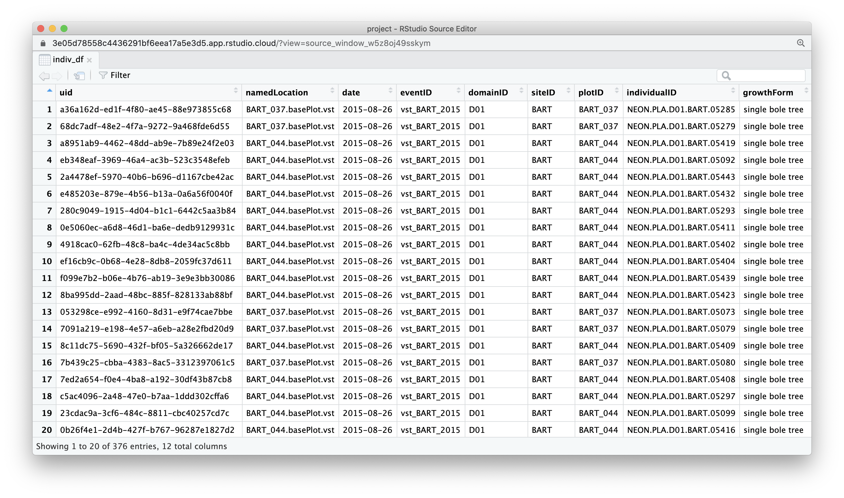

names(indiv_df)

 [1] "uid"               "namedLocation"     "date"             
 [4] "eventID"           "domainID"          "siteID"           
 [7] "plotID"            "individualID"      "growthForm"       
[10] "stemDiameter"      "measurementHeight" "height"

str(indiv_df)

spc_tbl_ [376 × 12] (S3: spec_tbl_df/tbl_df/tbl/data.frame)
 $ uid              : chr [1:376] "a36a162d-ed1f-4f80-ae45-88e973855c68" "68dc7adf-48e2-4f7a-9272-9a468fde6d55" "a8951ab9-4462-48dd-ab9e-7b89e24f2e03" "eb348eaf-3969-46a4-ac3b-523c3548efeb" ...
 $ namedLocation    : chr [1:376] "BART_037.basePlot.vst" "BART_037.basePlot.vst" "BART_044.basePlot.vst" "BART_044.basePlot.vst" ...
 $ date             : Date[1:376], format: "2015-08-26" "2015-08-26" ...
 $ eventID          : chr [1:376] "vst_BART_2015" "vst_BART_2015" "vst_BART_2015" "vst_BART_2015" ...
 $ domainID         : chr [1:376] "D01" "D01" "D01" "D01" ...
 $ siteID           : chr [1:376] "BART" "BART" "BART" "BART" ...
 $ plotID           : chr [1:376] "BART_037" "BART_037" "BART_044" "BART_044" ...
 $ individualID     : chr [1:376] "NEON.PLA.D01.BART.05285" "NEON.PLA.D01.BART.05279" "NEON.PLA.D01.BART.05419" "NEON.PLA.D01.BART.05092" ...
 $ growthForm       : chr [1:376] "single bole tree" "single bole tree" "single bole tree" "single bole tree" ...
 $ stemDiameter     : num [1:376] 17.1 13.7 12.3 12.1 29.2 12.1 23.4 39.5 10 10.6 ...
 $ measurementHeight: num [1:376] 130 130 130 130 130 130 130 130 130 130 ...
 $ height           : num [1:376] 15.2 9.8 7.7 15.2 16.7 10.6 18.4 19 5.7 8.7 ...
 - attr(*, "spec")=
  .. cols(
  ..   uid = col_character(),
  ..   namedLocation = col_character(),
  ..   date = col_date(format = ""),
  ..   eventID = col_character(),
  ..   domainID = col_character(),
  ..   siteID = col_character(),
  ..   plotID = col_character(),
  ..   individualID = col_character(),
  ..   growthForm = col_character(),
  ..   stemDiameter = col_double(),
  ..   measurementHeight = col_double(),
  ..   height = col_double()
  .. )
 - attr(*, "problems")=<externalptr>

summary(indiv_df)

     uid            namedLocation           date              eventID         
 Length:376         Length:376         Min.   :2015-08-26   Length:376        
 Class :character   Class :character   1st Qu.:2015-08-27   Class :character  
 Mode  :character   Mode  :character   Median :2015-08-27   Mode  :character  
                                       Mean   :2015-08-27                     
                                       3rd Qu.:2015-08-31                     
                                       Max.   :2015-08-31                     
   domainID            siteID             plotID          individualID      
 Length:376         Length:376         Length:376         Length:376        
 Class :character   Class :character   Class :character   Class :character  
 Mode  :character   Mode  :character   Mode  :character   Mode  :character  
                                                                            
                                                                            
                                                                            
  growthForm         stemDiameter   measurementHeight     height     
 Length:376         Min.   : 2.00   Min.   : 10.0     Min.   : 0.50  
 Class :character   1st Qu.:13.90   1st Qu.:130.0     1st Qu.:10.60  
 Mode  :character   Median :20.20   Median :130.0     Median :14.30  
                    Mean   :23.01   Mean   :129.5     Mean   :13.91  
                    3rd Qu.:29.55   3rd Qu.:130.0     3rd Qu.:17.23  
                    Max.   :69.90   Max.   :130.0     Max.   :30.20

skimr::skim(indiv_df)

Data summary
Name	indiv_df
Number of rows	376
Number of columns	12
_______________________
Column type frequency:
character	8
Date	1
numeric	3
________________________
Group variables	None

Variable type: character

skim_variable	n_missing	complete_rate	min	max	n_unique
uid	0	1.00	36	36	376
namedLocation	0	1.00	21	21	7
eventID	0	1.00	13	13	1
domainID	0	1.00	3	3	1
siteID	0	1.00	4	4	1
plotID	0	1.00	8	8	7
individualID	0	1.00	23	23	374
growthForm	3	0.99	7	16	4

Variable type: Date

skim_variable	n_missing	complete_rate	min	max	median	n_unique
date	0	1	2015-08-26	2015-08-31	2015-08-27	3

Variable type: numeric

skim_variable	complete_rate	mean	sd	p0	p25	p50	p75	p100	hist
stemDiameter	1	23.01	11.22	2.0	13.9	20.2	29.55	69.9	▆▇▃▁▁
measurementHeight	1	129.48	6.76	10.0	130.0	130.0	130.00	130.0	▁▁▁▁▇
height	1	13.91	4.45	0.5	10.6	14.3	17.22	30.2	▁▅▇▂▁

Update `individual.R`

Everything looks good. Before moving on, let’s update our individual.R script with the code we’ve just written and want to formally keep as part of out processing pipeline.

Add the following code and comments to the bottom of individual.R:

## code to prepare `individual` dataset goes here
## Setup ----
library(dplyr)

## Combine individual tables ----
# Create paths to inputs
raw_data_path <- here::here("data-raw", "wood-survey-data-master")
individual_paths <- fs::dir_ls(fs::path(raw_data_path, "individual"))

So let’s now move onto the next step of reading in all the files and combining them together. To do this, we’ll examine the principles of Iteration.

Reuse

CC BY-SA 4.0

Project Aims & Objectives

Project Aim

Project Objectives

Project Data

conventions: Data management

Setting up a data-raw/ directory

Download data

NEON Data

vst_perplotperyear: Plot level metadata, including plot geolocation.

vst_mappingandtagging: Mapping, identifying and tagging of individual stems for re-measurement.

vst_apparentindividual: Biomass and productivity measurements of apparent individuals.

Paths

Creating portable paths with here

Basic checks

Update individual.R

Reuse

Setting up a `data-raw/` directory

`vst_perplotperyear`: Plot level metadata, including plot geolocation.

`vst_mappingandtagging`: Mapping, identifying and tagging of individual stems for re-measurement.

`vst_apparentindividual`: Biomass and productivity measurements of apparent individuals.

Creating portable paths with `here`

Update `individual.R`