Creating a research compendium with rrtools

Research Compendia

Background

Research is increasingly computational
Code and data are important research outputs
- yet, we still focus mainly on curating papers.
Calls for openness
- stick: reproducibility crisis
- carrot: big rewards from working open

Yet we lag in conventions and technical infrastructure for such openness.

Enter the Research Compendium

The goal of a research compendium is to provide a standard and easily recognizable way for organizing the digital materials of a project to enable others to inspect, reproduce, and extend the research.

Three Generic Principles

Organize its files according to prevailing conventions:
- help other people recognize the structure of the project,
- supports tool building which takes advantage of the shared structure.
Separate of data, method, and output, while making the relationship between them clear.
Specify the computational environment that was used for the original analysis.

R community response

R packages can be used as a research compendium for organising and sharing files!

R package file system structure for reproducible research

Take advantage of the power of convention.
Make use of great package development tools.

See Ben Marwick, Carl Boettiger & Lincoln Mullen (2018) Packaging Data Analytical Work Reproducibly Using R (and Friends), The American Statistician, 72:1, 80-88, DOI: <10.1080/00031305.2017.1375986>

images: Kartik Ram: rstudio::conf 2019 talk — images: *Kartik Ram: rstudio::conf 2019 talk*

R Developer Tools

Leverage tools and functionality for R package development

manage dependencies
make functionality available
document functionality
validate functionality
version contol your project

devtools, usethis, rrtools, Rstudio

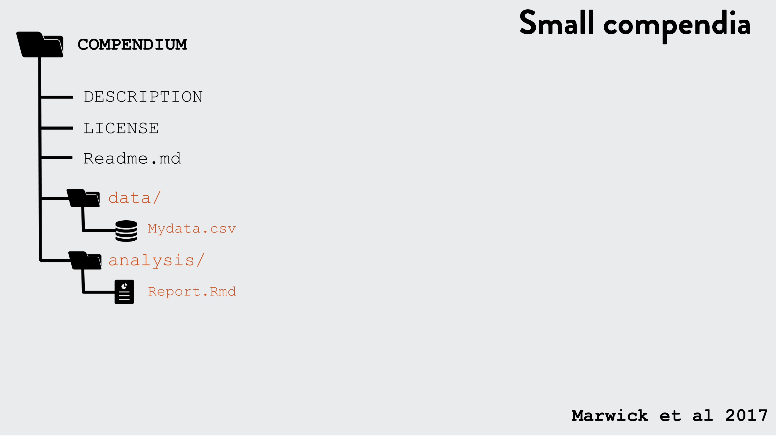
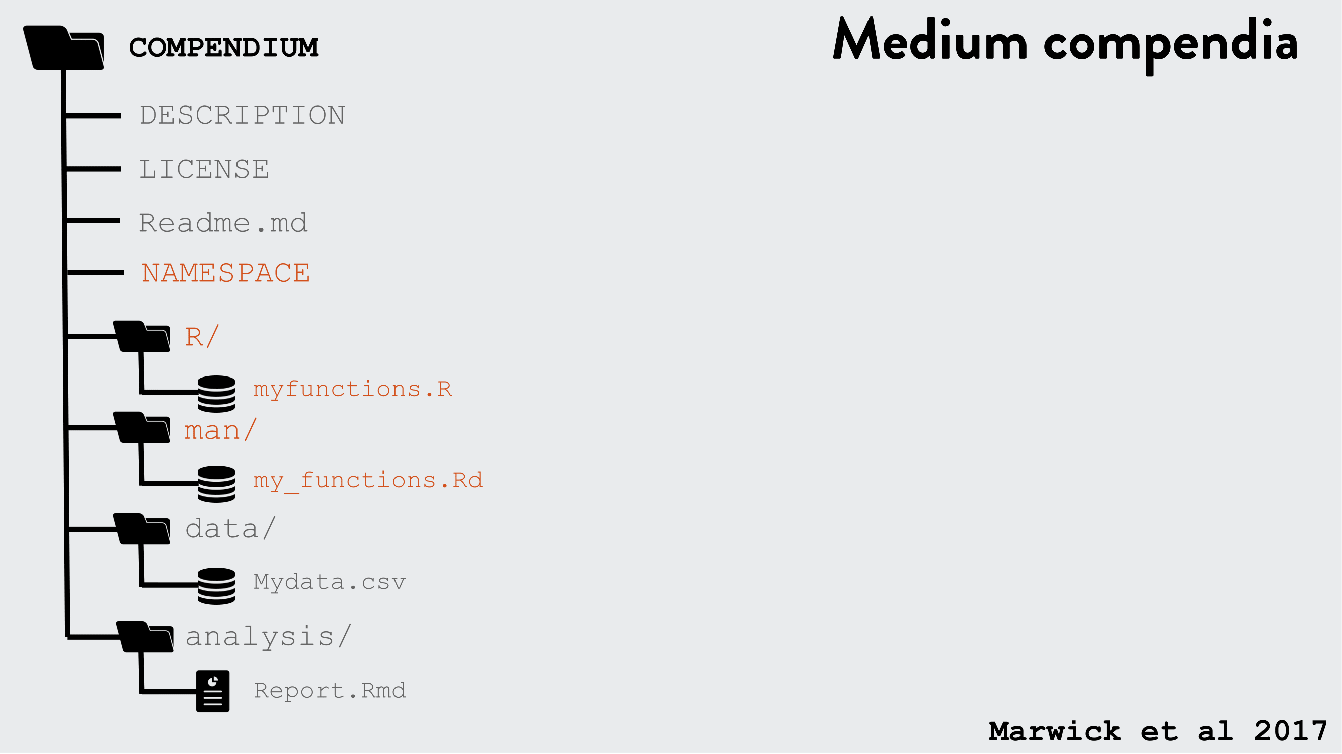
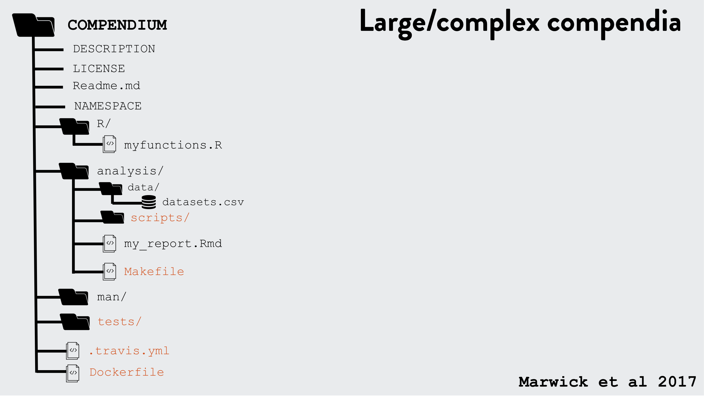
minimal analysis project

An scripts/ directory that contains R scripts (.R), notebooks (.qmd), and intermediate data.
A DESCRIPTION file that provides metadata about the compendium. Most importantly, it would list the packages needed to run the analysis. Would contain field to indicate that this is an analysis, not a package.

A reproducible analysis project might also contain:

An R/ directory which contains R files that provide high-stakes functions.
A data/ directory which contains high-stakes data.
A tests/ directory that contains unit tests for the code and data.
A vignettes/ directory that contains high-stakes reports.

Autogenerated components:

A man/ directory which contains roxygen2-generated documentation for the reusable functions and data.
Online documentation in a docs/ folder.

A shareable reproducible analysis project would also:

Use Git + GitHub (or other public Git host)
Use GitHub Actions or other continuous integration service
Capture the computational environment so it can easily be recreated on a different computer. This involves at a minimum capturing package versions, but might also include capturing R version, and other external dependencies.

Start small and build as necessary

`rrtools`: Research Compendia in R

The goal of rrtools is to provide instructions, templates, and functions for making a basic compendium suitable for writing reproducible research with R.

rrtools build on tools & conventions for R package development to

organise files
manage dependencies
share code
document code
check and test code

rrtools extends and works with a number of R packages:

devtools: functions for package development
usethis: automates repetitive tasks that arise during project setup and development
Quarto: facilitates writing of Scientific and Technical Documents.

Practical: Create a Research Compendium

Practical Aims and Objectives

In this section we’ll use materials associated with a published paper (text, data and code) to create a research compendium around it.

By the end of the workshop, you should be able to:

Create a Research Compendium to manage and share resources associated with an academic publication.
Produce a reproducible manuscript from a single rmarkdown document.
Appreciate the power of convention!

Create your first reproducible research compendium

Let’s go ahead and create our first reproducible research compendium!

Copy rrcompendium Project

In our shared space click on the copy button next to the rrcompendium Project.

The project already has the rrtools package and all the necessary dependencies installed.

Installing required packages locally

If you are working locally, you would need to install the following packages starting with rrtools.

# install rrtools
install.packages("remotes")
remotes::install_github("benmarwick/rrtools")

# install github dependencies
dependencies <- c("dplyr", "ggplot2", "ggthemes", "credentials", "Cairo")

# install CRAN dependencies
install.packages(dependencies)

# install tinytex
tinytex::install_tinytex()

You might also need to install tinytex (if you get errors when rendering your qmd paper).

Create compendium

Now that we’ve got a project to work in, let’s start by creating a blank research compendium for us to work in.

We use function rrtools::create_compendium.

Because we are already in the project we want to create the compendium in, we can just call the function without any arguments.

rrtools::create_compendium()

But see below for information on how to create a compendium locally in a new directory.

Creating a Research Compendium in a new directory locally

Locally we could supply a path at which our compendium will be created. The final part of our path becomes the compendium name. Because the function effectively creates a package, only a single string of lowercase alpha characters is accepted as a name, for example, rrcompendium as the final part of our path.

To create rrcompendium on my desktop I might use:

rrtools::create_compendium("~/Desktop/rrcompendium")

If the call was successfull you should see the following console output:

✔ Setting active project to '/cloud/project'
✔ Writing 'LICENSE'
✔ Writing 'LICENSE.md'
✔ Adding '^LICENSE\\.md$' to '.Rbuildignore'

✔ Creating 'README.Rmd' from template.
✔ Adding 'README.Rmd' to `.Rbuildignore`.
• Modify 
✔ Adding code of conduct.
✔ Creating 'CONDUCT.md' from template.
✔ Adding 'CONDUCT.md' to `.Rbuildignore`.
✔ Adding instructions to contributors.
✔ Creating 'CONTRIBUTING.md' from template.
✔ Adding 'CONTRIBUTING.md' to `.Rbuildignore`.
✔ Adding .binder/Dockerfile for Binder
✔ Creating '.binder'
✔ Creating '.binder/Dockerfile' from template.
✔ Adding '.binder/Dockerfile' to `.Rbuildignore`.
• Modify 

✔ Adding 'here' pkg to Imports
✔ Creating 'analysis' directory and contents
✔ Creating 'analysis'
✔ Creating 'analysis/paper'
✔ Creating 'analysis/figures'
✔ Creating 'analysis/templates'
✔ Creating 'analysis/data'
✔ Creating 'analysis/data/raw_data'
✔ Creating 'analysis/data/derived_data'
✔ Creating 'analysis/supplementary-materials'
✔ Creating 'references.bib' from template.
✔ Creating 'paper.qmd' from template.

Next, you need to:  ↓ ↓ ↓ ↓ 
• Write your article/report/thesis, start at the paper.qmd file
• Add the citation style library file (csl) to replace the default provided here, see https://github.com/citation-style-language/
• Add bibliographic details of cited items to the 'references.bib' file
• For adding captions & cross-referencing in an qmd, see https://quarto.org/docs/authoring/cross-references.html
• For adding citations & reference lists in an qmd, see https://quarto.org/docs/authoring/footnotes-and-citations.html

Note that:
⚠ Your data files are tracked by Git and will be pushed to GitHub 


This project was set up by rrtools.

You can start working now or apply some more basic configuration.
Check out https://github.com/benmarwick/rrtools for an explanation of all the project configuration functions of rrtools.

Initiate `git`

Let’s initialise our compendium with .git. We’ll need to configure git again as this is a new Rstudio cloud project.

# configure git
usethis::use_git_config(user.name = "Jane",
               user.email = "jane@example.org")
# intialise git and commit
usethis::use_git()

✔ Initialising Git repo
✔ Adding '.Rhistory', '.Rdata', '.httr-oauth', '.DS_Store', '.quarto' to '.gitignore'
There are 12 uncommitted files:
* '.binder/'
* '.gitignore'
* '.Rbuildignore'
* 'analysis/'
* 'CONDUCT.md'
* 'CONTRIBUTING.md'
* 'DESCRIPTION'
* 'LICENSE'
* 'LICENSE.md'
* 'NAMESPACE'
* ...
Is it ok to commit them?

1: No
2: Nope
3: Definitely

Selection:  3

Let’s agree to commit the files and also to restart Rstudio.

Let’s also change the default branch to the more modern convention of main instead of master. We can use usethis::git_default_branch_rename().

usethis::git_default_branch_rename()

ℹ Local branch 'master' appears to play the role of the default branch.
✔ Moving local 'master' branch to 'main'.
• Be sure to update files that refer to the default branch by name.
  Consider searching within your project for 'master'.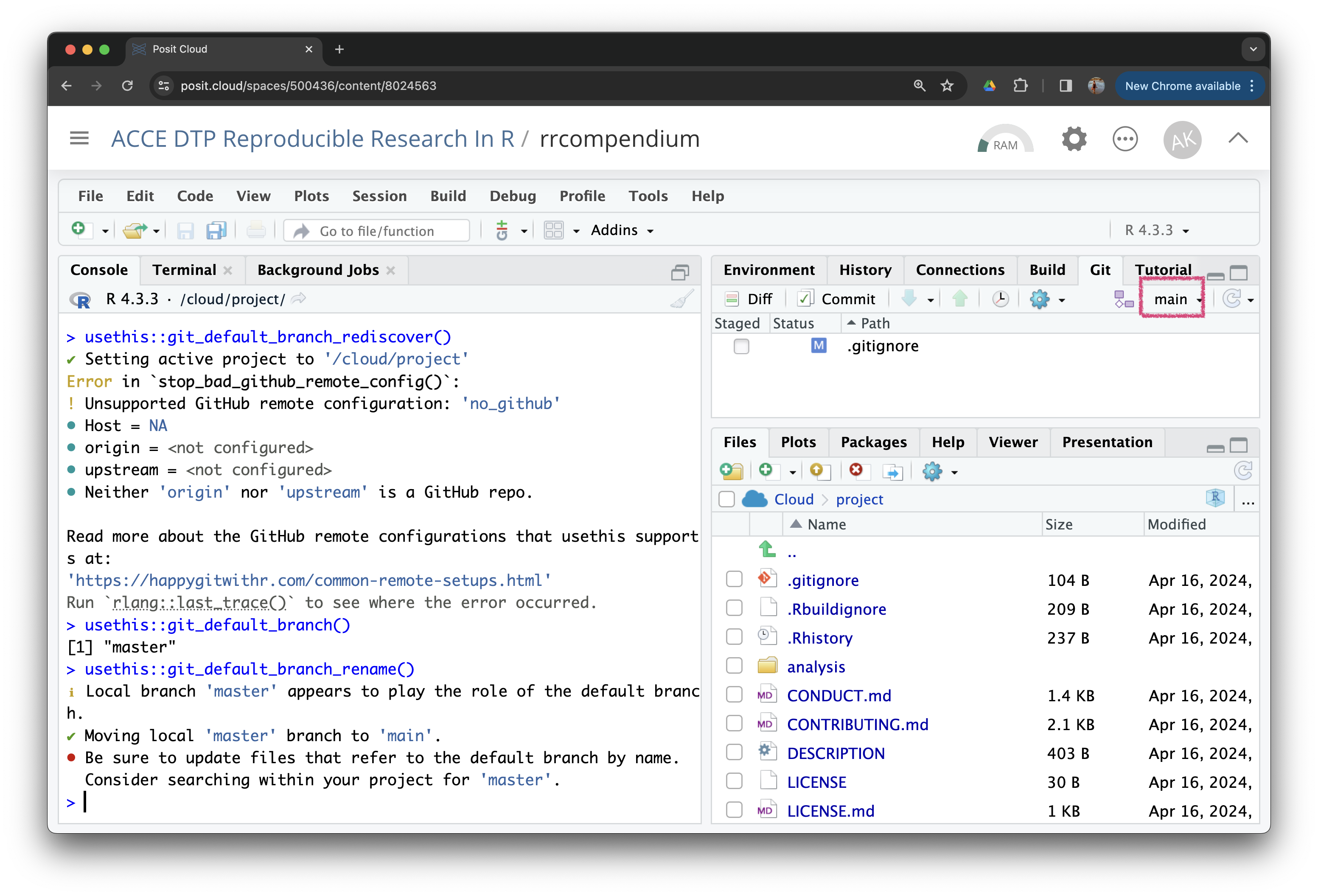

Inspect templates

rrtools::create_compendium() creates the bare backbone of infrastructure required for a research compendium. At this point it provides facilities to store general metadata about our compendium (eg bibliographic details to create a citation) and manage dependencies in the DESCRIPTION file and store and document functions in the R/ folder. Together these allow us to manage, install and share functionality associated with our project.

.
├── CONDUCT.md  <- .............................code of conduct
├── CONTRIBUTING.md <- .........................instructions for           
|                                               contributors
├── DESCRIPTION <- .............................package metadata
|                                               dependency management
├── LICENSE <- .................................license files
├── LICENSE.md
├── NAMESPACE <- ...............................AUTO-GENERATED on build
├── README.Rmd <- ..............................High level documentation
├── analysis
│   ├── data
│   │   ├── DO-NOT-EDIT-ANY-FILES-IN-HERE-BY-HAND
│   │   ├── derived_data
│   │   └── raw_data
│   ├── figures
│   ├── paper
│   │   ├── paper.qmd
│   │   └── references.bib
│   ├── supplementary-materials
│   └── templates
│       ├── author-info-blocks.lua
│       ├── journal-of-archaeological-science.csl
│       ├── pagebreak.lua
│       ├── scholarly-metadata.lua
│       ├── template.Rmd
│       └── template.docx
└── project.Rproj

Get session materials

Today we’ll be working with a subset of materials from the published compendium of code, data, and author’s manuscript:

Carl Boettiger. (2018, April 17). cboettig/noise-phenomena: Supplement to: “From noise to knowledge: how randomness generates novel phenomena and reveals information” (Version revision-2). Zenodo. http://doi.org/10.5281/zenodo.1219780

accompanying the publication:

Carl Boettiger . From noise to knowledge: how randomness generates novel phenomena and reveals information. Published in Ecology Letters, 22 May 2018 https://doi.org/10.1111/ele.13085

Create `attic` directory

Let’s first create a folder to dowload the materials into. It’s sometimes useful to have a folder to hold materials that are not formally part of the project (i.e. we will not commit these files to git). I like to call such folders attic, so let’s create such a folder

fs::dir_create("attic")

Let’s also add the attic/ dir to .gitignore and .buildignore (used to ignore files which should not be included as part of an installed R package) using usethis functions.

usethis::use_git_ignore("attic")

✔ Setting active project to
'/Users/Anna/Documents/workflows/workshops/rrresearch-acce-rrse'

usethis::use_build_ignore("attic")

Let’s also commit the changes to ,gitignore and .buildignore.

Download materials

You can download the materials using usethis::use_course() and supplying a path to a destination folder to argument destdir. Let’s download everything into the attic/ folder.

usethis::use_course(url = "bit.ly/rrtools_wks", destdir = "attic")

✔ Downloading from 'https://bit.ly/rrtools_wks'
Downloaded: 0.43 MB  
✔ Download stored in 'attic/rrtools-wkshp-materials-master.zip'
✔ Unpacking ZIP file into 'rrtools-wkshp-materials-master/' (7 files extracted)
Shall we delete the ZIP file ('rrtools-wkshp-materials-master.zip')?

1: Yes
2: Nope
3: Absolutely not

Selection: 
Enter an item from the menu, or 0 to exit
Selection: 1
✔ Deleting 'rrtools-wkshp-materials-master.zip'

This will download everything we need from a GitHub repository as a .zip file, unzip it and launch it in a new Rstudio session for us to explore.

Inspect materials

The follwing files should now be contained in your attic/rrtools-wkshp-materials-master folder

├── README.md <- .......................materials README
├── analysis.R <- ......................analysis underlying paper
├── gillespie.csv <- ...................data
├── paper.pdf <- .......................LaTex pdf of the paper
├── paper.txt <- .......................text body of the paper
└── refs.bib <- ........................bibtex bibliographic file

In this workshop we’ll attempt a partial reproduction of the original paper using the materials we’ve just downloaded.

We’ll use this as an opportunity to create a new research compendium using rrtools and friends! :confetti:

Update `DESCRIPTION` file

Let’s update some basic details in the DESCRIPTION file:

Package: project
Title: What the Package Does (One Line, Title Case)
Version: 0.0.0.9000
Authors@R:
    person("First", "Last", , "first.last@example.com", role = c("aut", "cre"))
Description: What the package does (one paragraph).
License: MIT + file LICENSE
ByteCompile: true
Encoding: UTF-8
LazyData: true
Roxygen: list(markdown = TRUE)
RoxygenNote: 7.3.1
Imports: here
Suggests: devtools,
    git2r

Package name

To get correct the limitation of working in Posit Cloud, were all projects are called project, let’s correct the Package: field and rename our package to rrcompendium.

Package: rrcompendium

Title

Let’s also give our compendium a descriptive title:

Title: Partial Reproduction of Boettiger Ecology Letters 2018;21:1255–1267 
    with rrtools

Version

We don’t need to change the version now but using semantic versioning for our compendium can be a really useful way to track versions. In general, versions below 0.0.1 are in development, hence the DESCRIPTION file defaults to 0.0.0.9000.

Authors

Next let’s specify the author of the compendium. Edit with your own details.

Authors@R: 
    person(given = "Anna",
           family = "Krystalli",
           role = c("aut", "cre"),
           email = "annakrystalli@googlemail.com")

For more details on specifying authors, check documentation for ?person

Description

Let’s add a bit more detail about the contents of the compendium in the Description.

Description: This repository contains the research compendium of the 
    partial reproduction of Boettiger Ecology Letters 2018;21:1255–1267. 
    The compendium contains all data, code, and text associated with this       sub-section of the analysis

Date

Add a Date field to the DESCRIPTION file to indicate when the compendium was created.

Date: 2024-04-19

License

Finally, let’s update the license for the material we create with copyright holder details. We’ll continue using the MIT license already created (Note however that his only covers the code). We can do this with:

usethis::use_mit_license("Anna Krystalli")

Overwrite pre-existing file 'LICENSE'?

1: No
2: Definitely
3: Not now

Selection: 2
✔ Writing 'LICENSE'
Overwrite pre-existing file 'LICENSE.md'?

1: Yup
2: Absolutely not
3: Not now

Selection: 1
✔ Writing 'LICENSE.md'

This overwrites the current files LICENSE and LICENSE.md and updates the DESCRIPTION file, embedding our name in the details of the license.

Recap

We’ve finished updating our DESCRIPTION file! 🎉

It should look a bit like this:

DESCRIPTION

Package: rrcompendium
Title: Partial Reproduction of Boettiger Ecology Letters 2018;21:1255–1267 
    with rrtools
Version: 0.0.0.9000
Authors@R: 
    person(given = "Anna",
           family = "Krystalli",
           role = c("aut", "cre"),
           email = "annakrystalli@googlemail.com")
Description: This repository contains the research compendium of the 
    partial reproduction of Boettiger Ecology Letters 2018;21:1255–1267. 
    The compendium contains all data, code, and text associated with this       
    sub-section of the analysis
License: MIT + file LICENSE
ByteCompile: true
Encoding: UTF-8
LazyData: true
Roxygen: list(markdown = TRUE)
RoxygenNote: 7.3.1
Date: 2024-04-19
Imports: here,
    dplyr (>= 1.1.4),
    fs (>= 1.6.3),
    ggplot2 (>= 3.5.0),
    ggthemes (>= 5.1.0),
    knitr (>= 1.46),
    readr (>= 2.1.5),
    rmarkdown (>= 2.26)
Suggests: devtools,
    git2r
URL: https://github.com/annakrystalli/rrcompendium
BugReports: https://github.com/annakrystalli/rrcompendium/issues

and your project folder should contain:

.
├── CONDUCT.md
├── CONTRIBUTING.md
├── DESCRIPTION
├── LICENSE
├── LICENSE.md
├── NAMESPACE
├── README.Rmd
├── analysis
│   ├── data
│   │   ├── DO-NOT-EDIT-ANY-FILES-IN-HERE-BY-HAND
│   │   ├── derived_data
│   │   └── raw_data
│   ├── figures
│   ├── paper
│   │   ├── paper.qmd
│   │   └── references.bib
│   ├── supplementary-materials
│   └── templates
│       ├── author-info-blocks.lua
│       ├── journal-of-archaeological-science.csl
│       ├── pagebreak.lua
│       ├── scholarly-metadata.lua
│       ├── template.Rmd
│       └── template.docx
├── attic
│   └── rrtools-wkshp-materials-master
│       ├── README.md
│       ├── analysis.R
│       ├── gillespie.csv
│       ├── paper.pdf
│       ├── paper.txt
│       └── refs.bib
└── project.Rproj

Let’s commit our work and move on to preparing our compendium for sharing on GitHub.

Create `paper.qmd` from template

When we first created our compendium, a paper.qmd file was created in the analysis/paper directory. This file is a template for a reproducible manuscript that we can use to write up our analysis and also serve to demonstrate how a reproducible paper should e set up.

However, the template is quite generic and we want to take advantage of the fact that Quarto offers templates for specific journals.

Given the original paper was published in Ecology Letters, an Elsevier journal, we’ll use the elsevier quarto template.

Delete current `paper/` directory

First, let’s delete the current paper/ directory and its contents.

fs::dir_delete("analysis/paper")

Create new `paper.qmd` from template

Next let’s move over to the Terminal and use the quarto CLI to create a new paper.qmd file from the elsevier template.

Terminal

quarto use template quarto-journals/elsevier

Quarto templates may execute code when documents are rendered. If you do not 
trust the authors of the template, we recommend that you do not install or 
use the template.
 ? Do you trust the authors of this template (Y/n) › Yes

When asked whether you trust the authors of the template, select Yes.

Next, you’ll be asked to provide a name for the new directory the new paper.qmd will be created in. Specify: analysis/paper.

Terminal

 ? Directory name: › analysis/paper

[✓] Downloading
[✓] Unzipping
    Found 1 extension.
[✓] Copying files...

Files created:
 - paper.qmd
 - placeholder.png
 - _extensions
 - bibliography.bib
 - style-guide

This creates the following files and directories in the analysis/paper directory:

analysis/paper
├── _extensions/
├── bibliography.bib
├── paper.qmd
├── placeholder.png
└── style-guide/

Copy materials into project

Let’s also copy some files we’ll be using in our project from the materials we downloaded into our attic/. In particular, we need to copy:

gillespie.csv (the paper data) into analysis/data
refs.bib (the paper references) into analysis/paper

We can do this programmatically using the fs package.

fs::file_copy(
  "attic/rrtools-wkshp-materials-master/gillespie.csv",
  "analysis/data"
)
fs::file_copy(
  "attic/rrtools-wkshp-materials-master/refs.bib",
  "analysis/paper"
)

Commit changes to the project.

Inspect `paper.qmd`

The paper.qmd file is a template for a reproducible manuscript that we can use to write up our analysis. It contains a lot of information about the features of the elsevier template and how to use it.

Let’s open the new paper.qmd file, take a look at the contents and render it.

Complete paper Front Matter

Let’s start by completing the front matter of the paper.qmd file.

Add title and author details

Let’s start with the title and author fields.

First delete the following lines:

title: Short Paper
subtitle: A Short Subtitle
author:
  - name: Alice Anonymous
    email: alice@example.com
    affiliations: 
        - id: some-tech
          name: Some Institute of Technology
          department: Department Name
          address: Street Address
          city: City
          state: State
          postal-code: Postal Code
    attributes:
        corresponding: true
    note: This is the first author footnote.
  - name: Bob Security
    email: bob@example.com
    affiliations:
        - id: another-u
          name: Another University
          department: Department Name
          address: Street Address
          city: City
          state: State
          postal-code: Postal Code
    note: |
      Another author footnote, this is a very long footnote and it should be a really long footnote. But this footnote is not yet sufficiently long enough to make two lines of footnote text.
  - name: Cat Memes
    email: cat@example.com
    affiliations:
        - ref: another-u
    note: Yet another author footnote.
  - name: Derek Zoolander
    email: derek@example.com
    affilations:
        - ref: some-tech

and replace them with information we can find in the downloaded materials, and in particular the paper.txt file. We’ll complete the information with the orginal author details.

title: "From noise to knowledge: how randomness generates novel phenomena and reveals information"
author:
  - name: "Carl Boettiger"
    email: "cboettig@berkeley.edu"
    affiliations: 
        - id: a
          address: "Dept of Environmental Science, Policy, and Management, University of California Berkeley, Berkeley CA 94720-3114, USA"
    attributes:
        corresponding: true

Add abstract and keywords

Next, let’s replace the abstract and keywords fields with the following. Again, we can find this information in the paper.txt file.

abstract: |
  Noise, as the term itself suggests, is most often seen a nuisance to ecological insight, a inconvenient reality that must be acknowledged, a haystack that must be stripped away to reveal the processes of interest underneath. Yet despite this well-earned reputation, noise is often interesting in its own right: noise can induce novel phenomena that could not be understood from some underlying determinstic model alone.  Nor is all noise the same, and close examination of differences in frequency, color or magnitude can reveal insights that would otherwise be inaccessible.  Yet with each aspect of stochasticity leading to some new or unexpected behavior, the time is right to move beyond the familiar refrain of "everything is important" (Bjørnstad & Grenfell 2001).  Stochastic phenomena can suggest new ways of inferring process from pattern, and thus spark more dialog between theory and empirical perspectives that best advances the field as a whole. I highlight a few compelling examples, while observing that the study of stochastic phenomena are only beginning to make this translation into empirical inference.  There are rich opportunities at this interface in the years ahead.
keywords: 
  - Coloured noise
  - demographic noise
  - environmental noise
  - quasi-cycles
  - stochasticity
  - tipping points

Change reference style to `authoryear`

Finally, in journal, let’s change the reference style to match the original paper by changinging cite-style to authoryear and set the name of the journal to Ecology Letters.

format:
  elsevier-pdf:
    keep-tex: true
    journal:
      name: Ecology Letters
      formatting: preprint
      model: 3p
      cite-style: authoryear

Complete paper body

Clear template content and paste text

Next, let’s clear the template body contents (everything outside the YAML Front Matter header) and paste the main text from paper.txt.

Copy everything between and including the # Introduction: ... and ## References sections in paper.txt and paste it into the paper.qmd file, below the YAML Front matter header.

Add Mathematical Notation

Through the ## Demographic stochasticity section of the paper, there is discussion simulation parameters that in the orginal paper are formatted using mathematical notations used for equations. To format such in-line text using such notation, surround it with $ dollar signs.

Here’s an example of what that looks like in paper.qmd:

 We summarize the myriad lower-level processes that
mechanistically lead to the event of a 'birth' in the population
as a probability: In a population of $N$ identical individuals at
time t, a birth occurs with probability $b_t(N_t)$ (_i.e._ a rate
that can depend on the population size, $N$), which increases the
population size to $N+1$. Similarly, death events occur with probability
$d_t(N_t)$, decreasing the population size by one individual, to $N-1$.

And what it looks like when rendered:

We summarize the myriad lower-level processes that mechanistically lead to the event of a ‘birth’ in the population as a probability: In a population of $N$ identical individuals at time t, a birth occurs with probability $b_t(N_t)$ (i.e. a rate that can depend on the population size, $N$), which increases the population size to $N+1$. Similarly, death events occur with probability $d_t(N_t)$, decreasing the population size by one individual, to $N-1$.

Read through that section and format any mathematical notation accordingly.

Update references

Next we’ll replace the flat citations in the text with real linked citation which can be used to auto-generate formatted in-line citations and the references section.

Add bibliography

To do this, first we’ll need to switch our bibliography to the refs.bib file. So in the YAML Front Matter, replace the bibliography field with the following:

bibliography: refs.bib

Insert citation cross-references

Firstly, to use the interactive citation features in Quarto, we need to move over to the Visual editor.

To many, stochasticity, or more simply, noise, is just that -- something which obscures patterns we are trying to infer [@Knape2011]; and an ever richer batteries of statistical methods are developed largely in an attempt to strip away this undesirable randomness to reveal the patterns beneath [@Coulson2001]. Over the past several decades, literature in stochasticity has transitioned from thinking of stochasticity in such terms; where noise is a nuisance that obscures the deterministic skeleton of the underlying mechanisms, to the recognition that stochasticity can itself be a mechanism for driving many interesting phenomena [@Coulson2004].

Commit changes

Add analysis code

Now that we’ve set up the text for our paper, the next step is to add the executable code that generates the figures in the paper. This code is provided in the analysis.R file in the materials we downloaded.

Inspect analysis.R file

Let’s also open analysis.R in the course materials and run the code. The script has some initial setup, then loads the data, recodes one of the columns for plotting and then plots the results of the simulation, which generates figure 1 in paper.pdf.

analysis.R

library(dplyr)
library(readr)
library(ggplot2)
library(ggthemes)
theme_set(theme_grey())
# create colour palette
colours <- ptol_pal()(2)

# load-data
data <- read_csv(here::here("gillespie.csv"), col_types = "cdiddd")

# recode-data
data <- data %>%
  mutate(system_size = recode(system_size,
                              large = "A. 1000 total sites",
                              small = "B. 100 total sites"))

# plot-gillespie
data %>%
  ggplot(aes(x = time)) +
  geom_hline(aes(yintercept = mean), lty=2, col=colours[2]) +
  geom_hline(aes(yintercept = minus_sd), lty=2, col=colours[2]) +
  geom_hline(aes(yintercept = plus_sd), lty=2, col=colours[2]) +
  geom_line(aes(y = n), col=colours[1]) +
  facet_wrap(~system_size, scales = "free_y")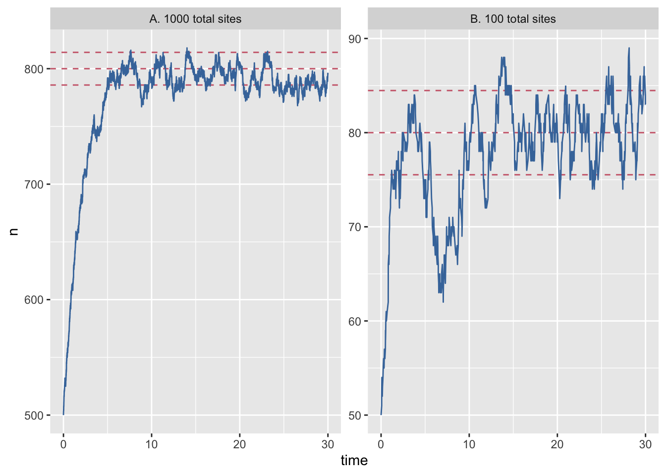

Let’s move back to our paper.qmd file and start adding the code to generate the plot.

Add document level code block configuration

Before we begin, let’s add some document level code block configuration which will apply to all code blocks in our document. We can do this by adding a knitr block to bottom of the YAML Front Matter of the paper.qmd file.

knitr:
  opts_block: 
    echo: false
    warning: false
    message: false

This sets the following options for all code blocks in the document: - echo: false suppresses the code output - warning: false suppresses warnings - message: false suppresses messages

Add block to load libraries

Next let’s insert a libraries code block right at the top of the document to set up our analysis. Because it’s a setup block we set #| include: false which suppresses all output resulting from block evaluation.

Add block to set plot themes

Right below the libraries block, insert a new block

Copy the code to set the plot theme and pasted into the block:

```{r}
theme_set(theme_grey())
```

Add `figure 1` block

Now scroll down towards the bottom of the document and create a new block just above the Conclusions section.

Add code

```{r}
# create colour palette
colours <- ptol_pal()(2)

# load-data
data <- read_csv(here::here("gillespie.csv"), col_types = "cdiddd")  

# recode-data
data <- data %>% 
  mutate(system_size = recode(system_size, large = "A. 1000 total sites", small= "B. 100 total sites")) 

# plot-gillespie
data %>%
  ggplot(aes(x = time)) + 
  geom_hline(aes(yintercept = mean), lty=2, col=colours[2]) + 
  geom_hline(aes(yintercept = minus_sd), lty=2, col=colours[2]) + 
  geom_hline(aes(yintercept = plus_sd), lty=2, col=colours[2]) + 
  geom_line(aes(y = n), col=colours[1]) +
  facet_wrap(~system_size, scales = "free_y") 
```

Edit path to data file to reflect the correct path to the data file in the project.

# load-data
data <- read_csv(here::here("analysis", "data", "gillespie.csv"), 
                 col_types = "cdiddd")

Add plot cross-reference

Next, to be able to cross-reference the plot in the text, we need to add a label to the block.

Let’s also add the figure caption found at the bottom of paper.txt to the plot through option fig-cap.

```{r}
#| label: fig-site-simulation
#| fig-cap: "Population dynamics from a Gillespie simulation of the Levins model with large (N=1000, panel A) and small (N=100, panel B) number of sites (blue) show relatively weaker effects of demographic noise in the bigger system. Models are otherwise identical, with e = 0.2 and c = 1 (code in appendix A). Theoretical predictions for mean and plus/minus one standard deviation shown in horizontal re dashed lines."
# create colour palette
colours <- ptol_pal()(2)

# load-data
data <- read_csv(here::here("analysis", "data", "gillespie.csv"), 
                 col_types = "cdiddd")

# recode-data
data <- data %>% 
  mutate(system_size = recode(system_size, large = "A. 1000 total sites", small= "B. 100 total sites")) 

# plot-gillespie
data %>%
  ggplot(aes(x = time)) + 
  geom_hline(aes(yintercept = mean), lty=2, col=colours[2]) + 
  geom_hline(aes(yintercept = minus_sd), lty=2, col=colours[2]) + 
  geom_hline(aes(yintercept = plus_sd), lty=2, col=colours[2]) + 
  geom_line(aes(y = n), col=colours[1]) +
  facet_wrap(~system_size, scales = "free_y") 
```

Now we can reference this plot in the text using @fig-site-simulation.

So let’s go ahead and replace:

Figure 1 shows the results of two exact SSA simulations of the classic patch model

with

@fig-site-simulation shows the results of two exact SSA simulations of the classic patch model

which will insert a clickable cross-reference to the plot in the text.

Find out more about adding cross-references to code block outputs in the Quarto documentation.

Commit changes

Capture Dependencies

Finally, before we’re finished, let’s ensure the dependencies introduced in the paper are captured. We can use rrtools::add_dependencies_to_description() to automatically detect and record the dependencies in the Imports section of our DESCRIPTION file.

rrtools::add_dependencies_to_description()

This will add the following to the DESCRIPTION file:

Imports: here,
    dplyr (>= 1.1.4),
    fs (>= 1.6.3),
    ggplot2 (>= 3.5.0),
    ggthemes (>= 5.1.0),
    knitr (>= 1.46),
    readr (>= 2.1.5),
    rmarkdown (>= 2.26)

and is a good start because it records any packages needed as well as a minimum version required. To ensure these packages are installed, another user of our project could just run install.packages("remotes") and then remotes::install_deps() to install all the dependencies listed in the DESCRIPTION file.

However, this does not guarantee and exact version of packages so breaking changes in new versions of packages could cause issues. To ensure exact versions are recorded, we can use renv again to create a snapshot of the project library. In fact we can combine the information contained in the DESCRIPTION file with the snapshot with renv to create an explicit lockfile that tracks the imports listed in DESCRIPTION.

Let’s start by initialising renv in our project.

renv::init()

Because it detects a DESCRIPTION file, renv will ask us how to proceed. Select 1: Use only the DESCRIPTION file. (explicit mode).

This project contains a DESCRIPTION file.
Which files should renv use for dependency discovery in this project? 

1: Use only the DESCRIPTION file. (explicit mode)
2: Use all files in this project. (implicit mode)

Once selected, renv will proceed to create a lockfile that captures the exact versions of the packages listed in DESCRIPTION in the project library.

- Using 'explicit' snapshot type. Please see `?renv::snapshot` for more details.

- Linking packages into the project library ... [113/113] Done!
- Resolving missing dependencies ... 
# Downloading packages --------------------------------------------
- Downloading devtools from CRAN ...            OK [417.5 Kb]
- Downloading fs from CRAN ...                  OK [281.2 Kb]
- Downloading rmarkdown from CRAN ...           OK [2.5 Mb]
- Downloading knitr from CRAN ...               OK [1007.1 Kb]
- Downloading roxygen2 from CRAN ...            OK [697.9 Kb in 0.17s]
- Downloading dplyr from CRAN ...               OK [1.4 Mb]
- Downloading ggplot2 from CRAN ...             OK [4.6 Mb]
- Downloading ggthemes from CRAN ...            OK [425.5 Kb in 0.12s]
- Downloading git2r from CRAN ...               OK [425 Kb in 0.38s]
- Downloading here from CRAN ...                OK [51.5 Kb]
- Downloading readr from CRAN ...               OK [864.8 Kb]
Successfully downloaded 11 packages in 3.2 seconds.

# Installing packages ---------------------------------------------
- Installing fs ...                             OK [installed binary and cached in 0.55s]
- Installing knitr ...                          OK [installed binary and cached in 0.53s]
- Installing rmarkdown ...                      OK [installed binary and cached in 0.74s]
- Installing roxygen2 ...                       OK [installed binary and cached in 0.66s]
- Installing devtools ...                       OK [installed binary and cached in 1.0s]
- Installing dplyr ...                          OK [installed binary and cached in 0.73s]
- Installing ggplot2 ...                        OK [installed binary and cached in 0.99s]
- Installing ggthemes ...                       OK [installed binary and cached in 0.86s]
- Installing git2r ...                          OK [installed binary and cached in 0.4s]
- Installing here ...                           OK [installed binary and cached in 0.37s]
- Installing readr ...                          OK [installed binary and cached in 0.67s]
The following package(s) will be updated in the lockfile:

# CRAN ------------------------------------------------------------
- dplyr          [* -> 1.1.4]
- fs             [* -> 1.6.3]
- ggplot2        [* -> 3.5.0]
- ggthemes       [* -> 5.1.0]
- here           [* -> 1.0.1]
- knitr          [* -> 1.46]
- lattice        [* -> 0.22-5]
- MASS           [* -> 7.3-60.0.1]
- Matrix         [* -> 1.6-5]
- mgcv           [* -> 1.9-1]
- nlme           [* -> 3.1-164]
- readr          [* -> 2.1.5]
- rmarkdown      [* -> 2.26]

# RSPM ------------------------------------------------------------
- base64enc      [* -> 0.1-3]
- bit            [* -> 4.0.5]
- bit64          [* -> 4.0.5]
- bslib          [* -> 0.7.0]
- cachem         [* -> 1.0.8]
- cli            [* -> 3.6.2]
- clipr          [* -> 0.8.0]
- colorspace     [* -> 2.1-0]
- cpp11          [* -> 0.4.7]
- crayon         [* -> 1.5.2]
- digest         [* -> 0.6.35]
- evaluate       [* -> 0.23]
- fansi          [* -> 1.0.6]
- farver         [* -> 2.1.1]
- fastmap        [* -> 1.1.1]
- fontawesome    [* -> 0.5.2]
- generics       [* -> 0.1.3]
- glue           [* -> 1.7.0]
- gtable         [* -> 0.3.4]
- highr          [* -> 0.10]
- hms            [* -> 1.1.3]
- htmltools      [* -> 0.5.8.1]
- isoband        [* -> 0.2.7]
- jquerylib      [* -> 0.1.4]
- jsonlite       [* -> 1.8.8]
- labeling       [* -> 0.4.3]
- lifecycle      [* -> 1.0.4]
- magrittr       [* -> 2.0.3]
- memoise        [* -> 2.0.1]
- mime           [* -> 0.12]
- munsell        [* -> 0.5.1]
- pillar         [* -> 1.9.0]
- pkgconfig      [* -> 2.0.3]
- prettyunits    [* -> 1.2.0]
- progress       [* -> 1.2.3]
- purrr          [* -> 1.0.2]
- R6             [* -> 2.5.1]
- rappdirs       [* -> 0.3.3]
- RColorBrewer   [* -> 1.1-3]
- renv           [* -> 1.0.7]
- rlang          [* -> 1.1.3]
- rprojroot      [* -> 2.0.4]
- sass           [* -> 0.4.9]
- scales         [* -> 1.3.0]
- stringi        [* -> 1.8.3]
- stringr        [* -> 1.5.1]
- tibble         [* -> 3.2.1]
- tidyselect     [* -> 1.2.1]
- tinytex        [* -> 0.50]
- tzdb           [* -> 0.4.0]
- utf8           [* -> 1.2.4]
- vctrs          [* -> 0.6.5]
- viridisLite    [* -> 0.4.2]
- vroom          [* -> 1.6.5]
- withr          [* -> 3.0.0]
- xfun           [* -> 0.43]
- yaml           [* -> 2.3.8]

The version of R recorded in the lockfile will be updated:
- R              [* -> 4.3.3]

- Lockfile written to "/cloud/project/renv.lock".

Commit changes

Update README

Every GitHub repository needs a README landing page.

When we intialised our research compendium, an rrtools README template was created.

It contains:

details of authorship and DOI of the associated paper.
details of authorship and DOI of the code and data.
a template citation to show others how to cite your project.
instructions on how to download and install the compendium
instructions on how to reproduce the analysis
license information for the text, figures, code and data in your compendium

The call also created two other community facing markdown files:

CONDUCT.md: a code of conduct for users
CONTRIBUTING.md: basic instructions for people who want to contribute to our compendium

Tip

You can always re-create an rrtools style README with:

rrtools::use_readme_rmd()

update `README`

There’s 5 main edits we need to make to the template:

Add title

In the first code block, assign the title to the title object:

Title <- "Partial Reproduction of Boettiger Ecology Letters 2018;21:1255–1267 with rrtools"

Edit author and year details

Where details of authors are requested, add your own name and year.

We don’t have a link to the DOI or details of where our partial reproduction is published so just leave as is.

Adjust installation instructions

Since we’re using renv to manage our dependencies, we need to update the installation instructions to reflect this. So replace the instruction to run devtools::install() with the following renv::restore()

Replace any mention of `paper.docx` to `paper.pdf`.

The original compendium template assumes the paper is in .docx format. We have changed ours to default to a .pdf so we need to update the installation instructions to reflect this.

Adjust data LICENSE

Let’s adjust the data LICENSE to match the source compendium license, which is CC-BY 4.0. Let’s also add Carl Boettiger as copyright holder of the data.

**Text and figures :**  [CC-BY-4.0](http://creativecommons.org/licenses/by/4.0/), Copyright (c) 2018 Carl Boettiger.

**Code :** See the [DESCRIPTION](DESCRIPTION) file

**Data :** [CC-BY-4.0](http://creativecommons.org/licenses/by/4.0/), Copyright (c) 2018 Carl Boettiger.

Remember to knit your README.Rmd to it’s .md version.

Commit changes

Create GitHub repository

Next, we’ll create a GitHub repository to share our compendium. We’ll make use of our GITHUB_PAT again so we will need to set up credentials again in this new project!

# configure GitHub PAT credentials
credentials::set_github_pat()

When working locally, away from the Posit Cloud limitation of all projects being called project, you can use usethis::use_github() to create a new repository on GitHub like we did for our wood-survey project.

# create GitHub repository and push
usethis::use_github(protocol = "https")

However, because we have already got a repository called project on GitHub, use_github() fails. So, I’ll show you another way to create a repository and push our project to it that will allow us to use a different name.

Create a new repository on GitHub manually

Navigate to your GitHub account, click on Repositories and the click the button New:

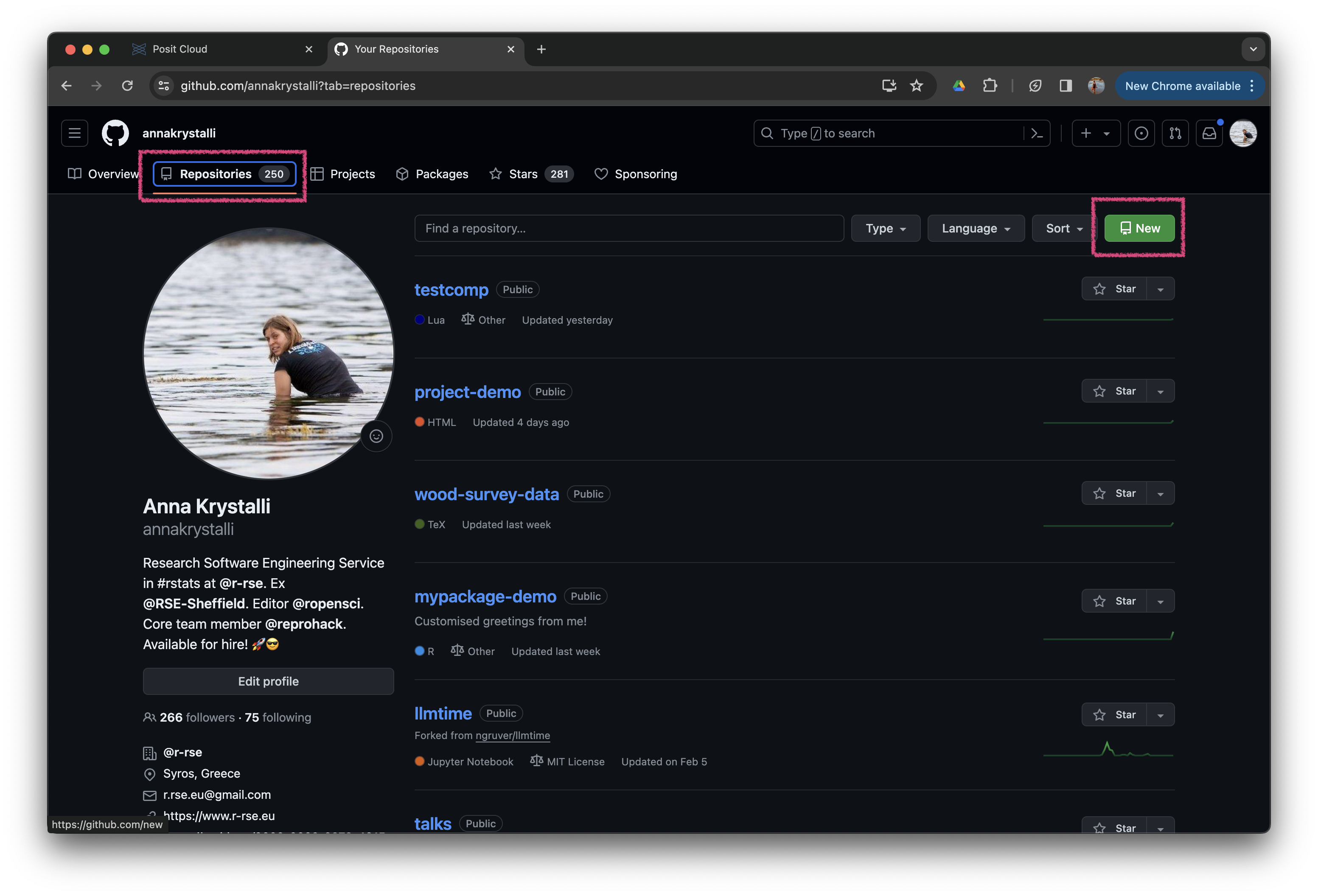
Next add the name for your repository, rrcompendium and make sure to set an owner if necessary. Don’t change anything else, just scroll to the bottom and click Create repository.

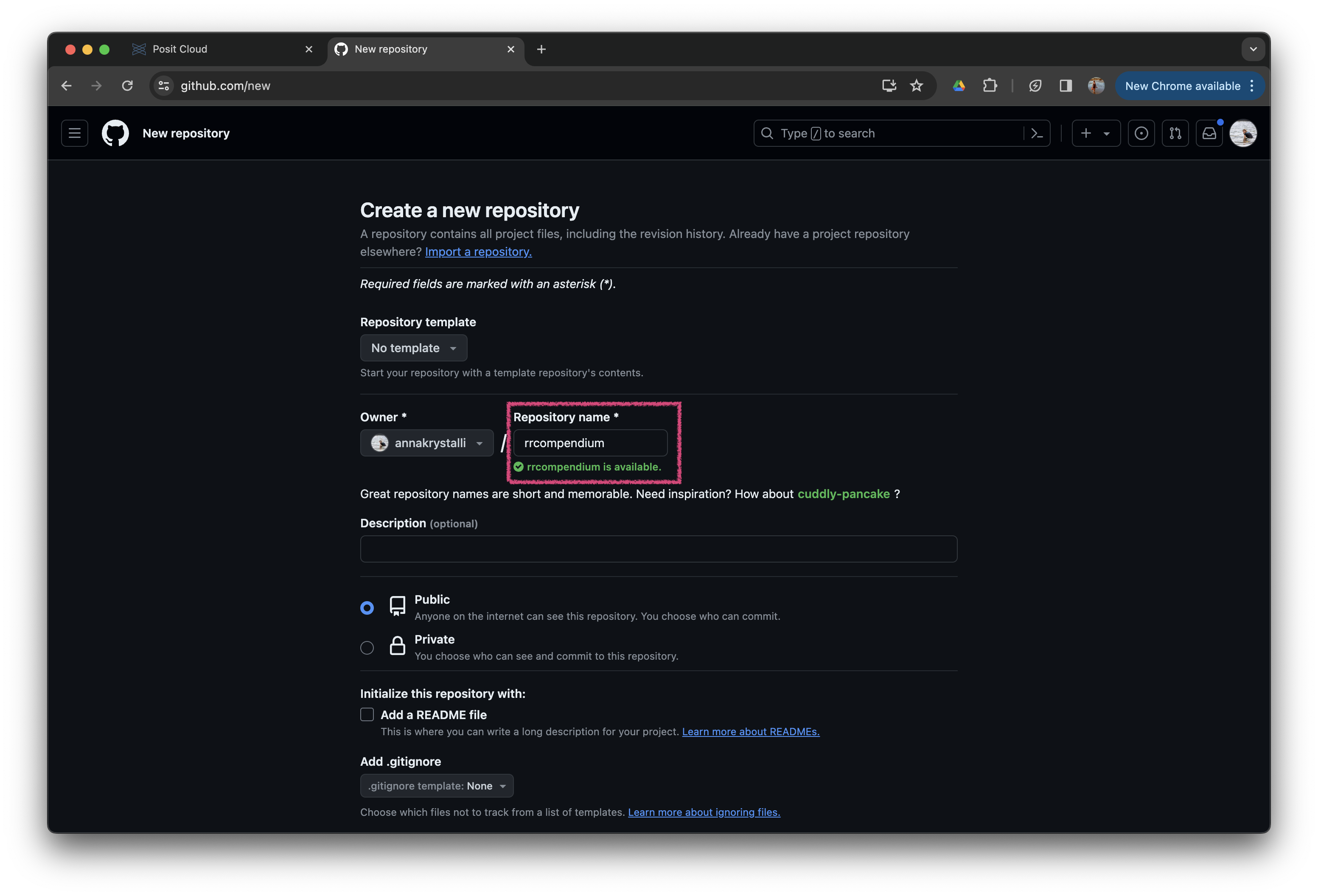This will create a completely empty new repository on GitHub called rrcompendium.

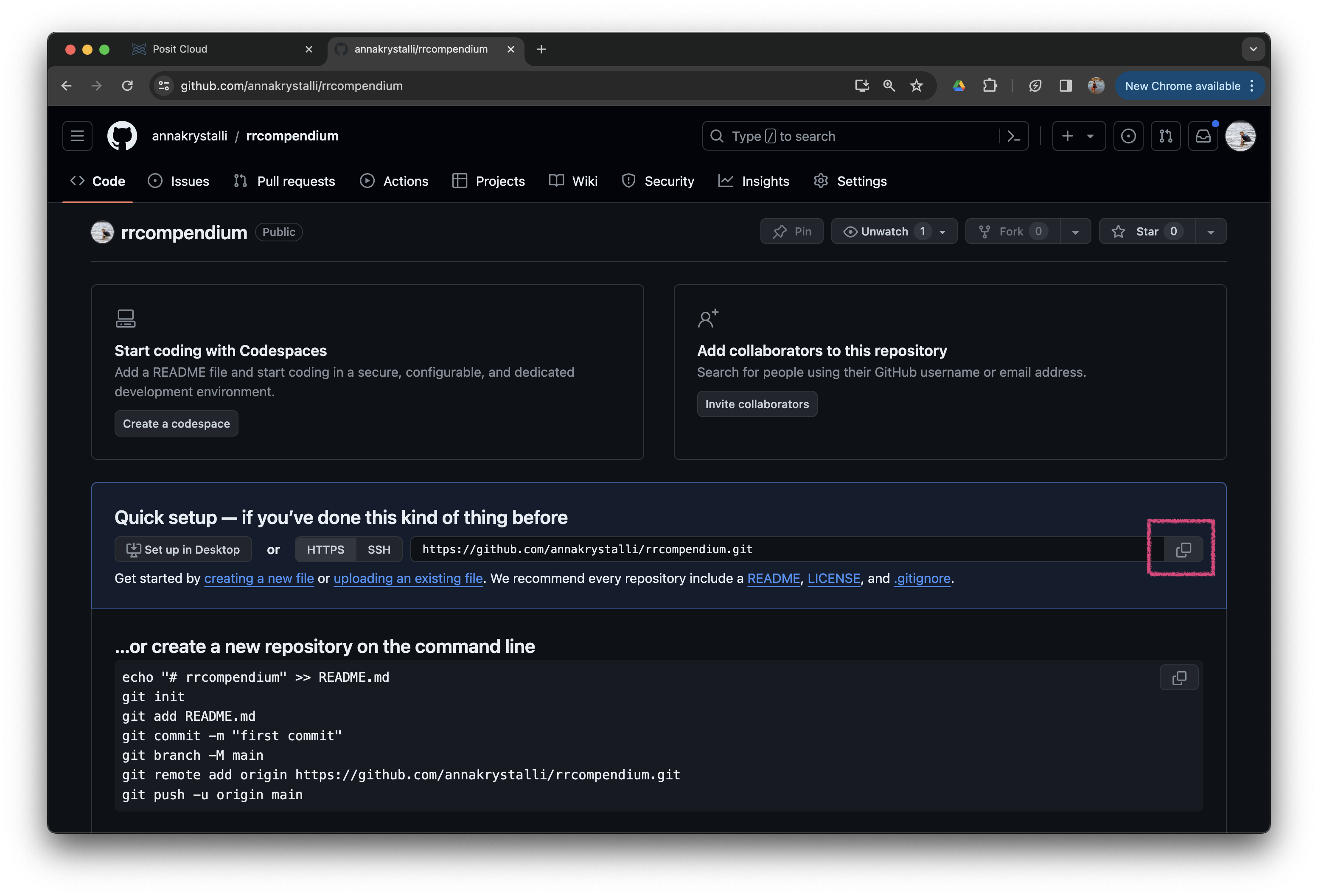
Copy the repository URL

Next, copy the URL of the repository from the Quick Setup box by clicking on the copy button next to the URL.

Add remote in Posit Cloud project

To add the repository we just created on GitHub as the origin remote in our project, we can use usethis::use_git_remote().

Supply the URL you copied from the GitHub repository you just created as argument url, e.g.:

usethis::use_git_remote(
  name = "origin",
  url = "https://github.com/annakrystalli/rrcompendium.git")

This will add the remote repository as the origin remote in our project.

Create remote `main` branch and push

Finally, let’s create a remote main branch in our project to track our local main branch and push our project to GitHub.

To do this, we’ll need to use the Terminal again and run the following commands:

Terminal

git push -u origin main

This will push our project to the main branch of the repository we created on GitHub.

Add GitHub links to DESCRIPTION

Finally, let’s add the GitHub repository link to the DESCRIPTION file so that others can easily access the project.

usethis::use_github_links()

Final Compendium

You can browse a demo of the final compendium here

Reuse

CC BY-SA 4.0

Background

Enter the Research Compendium

Three Generic Principles

R community response

R package file system structure for reproducible research

R Developer Tools

Leverage tools and functionality for R package development

minimal analysis project

A reproducible analysis project might also contain:

Autogenerated components:

A shareable reproducible analysis project would also:

Start small and build as necessary

rrtools: Research Compendia in R

Practical: Create a Research Compendium

Practical Aims and Objectives

Create your first reproducible research compendium

Copy rrcompendium Project

Create compendium

Initiate git

Inspect templates

Get session materials

Create attic directory

Download materials

Inspect materials

Update DESCRIPTION file

Package name

Title

Version

Authors

Description

Date

License

Recap

Create paper.qmd from template

Delete current paper/ directory

Create new paper.qmd from template

Copy materials into project

Inspect paper.qmd

Complete paper Front Matter

Add title and author details

Add abstract and keywords

Change reference style to authoryear

Complete paper body

Clear template content and paste text

Add Mathematical Notation

Update references

Add bibliography

Insert citation cross-references

Commit changes

Add analysis code

Inspect analysis.R file

Add document level code block configuration

Add block to load libraries

Add block to set plot themes

Add figure 1 block

Add code

Add plot cross-reference

Commit changes

Capture Dependencies

Commit changes

Sharing a compendium on GitHub

Update README

update README

Add title

Edit author and year details

Adjust installation instructions

Replace any mention of paper.docx to paper.pdf.

Adjust data LICENSE

Commit changes

Create GitHub repository

Create a new repository on GitHub manually

Copy the repository URL

Add remote in Posit Cloud project

Create remote main branch and push

Add GitHub links to DESCRIPTION

Final Compendium

Reuse

`rrtools`: Research Compendia in R

Initiate `git`

Create `attic` directory

Update `DESCRIPTION` file

Create `paper.qmd` from template

Delete current `paper/` directory

Create new `paper.qmd` from template

Inspect `paper.qmd`

Change reference style to `authoryear`

Add `figure 1` block

update `README`

Replace any mention of `paper.docx` to `paper.pdf`.

Create remote `main` branch and push