for (i in 1:10) {
  print(paste0("i is ", i))
}
[1] "i is 1"
[1] "i is 2"
[1] "i is 3"
[1] "i is 4"
[1] "i is 5"
[1] "i is 6"
[1] "i is 7"
[1] "i is 8"
[1] "i is 9"
[1] "i is 10"![]()
Data Munging
Let’s say we want to repeat a process multiple times, iterating over a number of inputs. In this case we want to load every file in data-raw/wood-survey-data-master/individual/.
We have a few options for how to approach this problem. In R there are two paradigms for iteration:
for loop.Here’s an example of a simple loop. During each iteration, it prints a message to the console, reporting the value of i.
for (i in 1:10) {
print(paste0("i is ", i))
}[1] "i is 1"
[1] "i is 2"
[1] "i is 3"
[1] "i is 4"
[1] "i is 5"
[1] "i is 6"
[1] "i is 7"
[1] "i is 8"
[1] "i is 9"
[1] "i is 10"The loop iterates over the vector of values supplied in 1:10, sequentially assigning a new value to variable i each iteration. i is therefore the varying input and everything else in the code stays the same during each iteration.
Let’s now apply a loop to read in all 67 files at once.
We have the file paths in our individual_paths vector. This is the input we want to iterate over. We can use a for loop to supply each path as the file argument in readr::read_csv().
The previous loop we saw didn’t generate any new objects, it just printed output to the console. We, however, need to store the output of each iteration (the tibble we’ve just read in).
It’s important for efficiency to allocate sufficient space in memory for the output before starting a for loop. Growing the for loop at each iteration, using c() for example, will be very slow.
Let’s create an output vector to store the tibbles containing the read in data. We want it to be a list because we’ll be storing heterogeneous objects (tibbles) in each element.
indiv_df_list <- vector("list", length(individual_paths))

head(indiv_df_list)
[[1]]
NULL
[[2]]
NULL
[[3]]
NULL
[[4]]
NULL
[[5]]
NULL
[[6]]
NULLWe’ve used the length() of the input to specify the size of our output list so each path gets an output element.
Next, we need a sequence of indices as long as the input vector (individual_paths). We can use seq_along() to create our index vector:
seq_along(individual_paths) [1] 1 2 3 4 5 6 7 8 9 10 11 12 13 14 15 16 17 18 19 20 21 22 23 24 25
[26] 26 27 28 29 30 31 32 33 34 35 36 37 38 39 40 41 42 43 44 45 46 47 48 49 50
[51] 51 52 53 54 55 56 57 58 59 60 61 62 63 64 65 66 67Now we’re ready to write our for loop.
for (i in seq_along(individual_paths)) {
  indiv_df_list[[i]] <- readr::read_csv(individual_paths[i], show_col_types = FALSE)
}
At each step of the iteration, the file specified in the ith element of individual_paths vector is read in and assigned to th ith element of our output list.
We’re also using the show_col_types argument to read_csv() to suppress the output of column types to the console.
We can extract individual tibbles using [[ sub-setting to inspect:
indiv_df_list[[1]]# A tibble: 376 × 12
uid namedLocation date eventID domainID siteID plotID individualID
<chr> <chr> <date> <chr> <chr> <chr> <chr> <chr>
1 a36a162… BART_037.bas… 2015-08-26 vst_BA… D01 BART BART_… NEON.PLA.D0…
2 68dc7ad… BART_037.bas… 2015-08-26 vst_BA… D01 BART BART_… NEON.PLA.D0…
3 a8951ab… BART_044.bas… 2015-08-26 vst_BA… D01 BART BART_… NEON.PLA.D0…
4 eb348ea… BART_044.bas… 2015-08-26 vst_BA… D01 BART BART_… NEON.PLA.D0…
5 2a4478e… BART_044.bas… 2015-08-26 vst_BA… D01 BART BART_… NEON.PLA.D0…
6 e485203… BART_044.bas… 2015-08-26 vst_BA… D01 BART BART_… NEON.PLA.D0…
7 280c904… BART_044.bas… 2015-08-26 vst_BA… D01 BART BART_… NEON.PLA.D0…
8 0e5060e… BART_044.bas… 2015-08-26 vst_BA… D01 BART BART_… NEON.PLA.D0…
9 4918cac… BART_044.bas… 2015-08-26 vst_BA… D01 BART BART_… NEON.PLA.D0…
10 ef16cb9… BART_044.bas… 2015-08-26 vst_BA… D01 BART BART_… NEON.PLA.D0…
# ℹ 366 more rows
# ℹ 4 more variables: growthForm <chr>, stemDiameter <dbl>,
# measurementHeight <dbl>, height <dbl>indiv_df_list[[2]]# A tibble: 714 × 12
uid namedLocation date eventID domainID siteID plotID individualID
<chr> <chr> <date> <chr> <chr> <chr> <chr> <chr>
1 fb75a8c… BART_036.bas… 2015-09-01 vst_BA… D01 BART BART_… NEON.PLA.D0…
2 30a7c77… BART_046.bas… 2015-09-01 vst_BA… D01 BART BART_… NEON.PLA.D0…
3 789d030… BART_072.bas… 2015-09-01 vst_BA… D01 BART BART_… NEON.PLA.D0…
4 0e4fb38… BART_072.bas… 2015-09-01 vst_BA… D01 BART BART_… NEON.PLA.D0…
5 cb0e456… BART_036.bas… 2015-09-01 vst_BA… D01 BART BART_… NEON.PLA.D0…
6 5fc5cf8… BART_072.bas… 2015-09-01 vst_BA… D01 BART BART_… NEON.PLA.D0…
7 5d15faf… BART_046.bas… 2015-09-01 vst_BA… D01 BART BART_… NEON.PLA.D0…
8 d27a1bf… BART_036.bas… 2015-09-01 vst_BA… D01 BART BART_… NEON.PLA.D0…
9 d5f9ab5… BART_036.bas… 2015-09-01 vst_BA… D01 BART BART_… NEON.PLA.D0…
10 e52c3be… BART_036.bas… 2015-09-01 vst_BA… D01 BART BART_… NEON.PLA.D0…
# ℹ 704 more rows
# ℹ 4 more variables: growthForm <chr>, stemDiameter <dbl>,
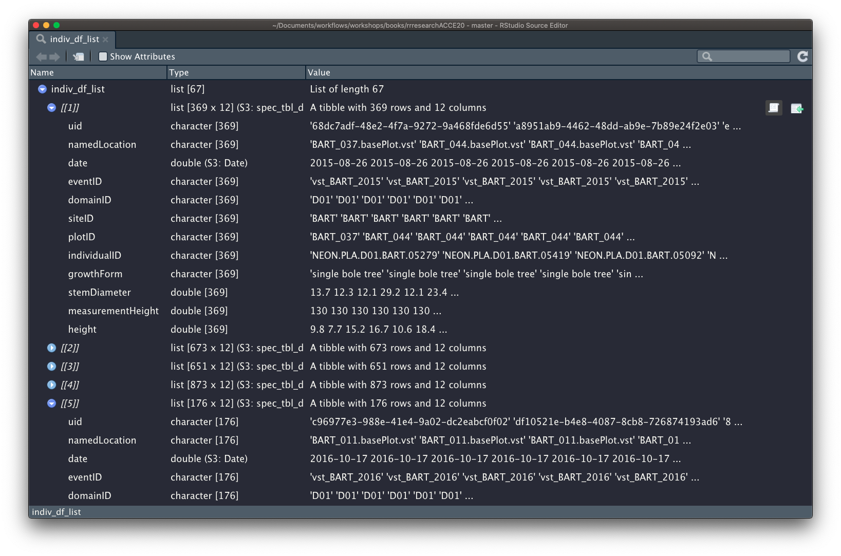
# measurementHeight <dbl>, height <dbl>We can also inspect the contents of our output list interactively using View()
We can also loop over objects instead of indices.
In this case, we’ll supply the paths themselves as the input to our loop and these will be passed as-is to read_csv().
This time we don’t have our element indices to index the elements of the output list each tibble should be stored in. To get around this we’ll assign names to each element and index the output list by name.
We can use the basename (actual file name) of each path as a name, which I can get through basename() from each file path.
individual_paths[1]
basename(individual_paths[1])/cloud/project/data-raw/wood-survey-data-master/individual/NEON.D01.BART.DP1.10098.001.vst_apparentindividual.2015-08.basic.20190806T172340Z.csv[1] "NEON.D01.BART.DP1.10098.001.vst_apparentindividual.2015-08.basic.20190806T172340Z.csv"So let’s tweak our output list to store the tibbles by name rather than index.
1indiv_df_list <- vector("list", length(individual_paths))
2names(indiv_df_list) <- basename(individual_paths)individual_paths.
basename of each path as the name of each element in the output list.
Let’s have a look at the first few elements of our output list:
head(indiv_df_list)$`NEON.D01.BART.DP1.10098.001.vst_apparentindividual.2015-08.basic.20190806T172340Z.csv`
NULL
$`NEON.D01.BART.DP1.10098.001.vst_apparentindividual.2015-09.basic.20190806T144119Z.csv`
NULL
$`NEON.D01.BART.DP1.10098.001.vst_apparentindividual.2016-08.basic.20190806T143255Z.csv`
NULL
$`NEON.D01.BART.DP1.10098.001.vst_apparentindividual.2016-09.basic.20190806T143433Z.csv`
NULL
$`NEON.D01.BART.DP1.10098.001.vst_apparentindividual.2016-10.basic.20190806T144133Z.csv`
NULL
$`NEON.D01.BART.DP1.10098.001.vst_apparentindividual.2017-07.basic.20190806T144111Z.csv`
NULLNow we can loop over the paths themselves:
1for (path in individual_paths) {
2 indiv_df_list[[basename(path)]] <- readr::read_csv(path, show_col_types = FALSE)
}path during each iteration.
head(indiv_df_list, 2)$`NEON.D01.BART.DP1.10098.001.vst_apparentindividual.2015-08.basic.20190806T172340Z.csv`
# A tibble: 376 × 12
   uid      namedLocation date       eventID domainID siteID plotID individualID
   <chr>    <chr>         <date>     <chr>   <chr>    <chr>  <chr>  <chr>
 1 a36a162… BART_037.bas… 2015-08-26 vst_BA… D01      BART   BART_… NEON.PLA.D0…
 2 68dc7ad… BART_037.bas… 2015-08-26 vst_BA… D01      BART   BART_… NEON.PLA.D0…
 3 a8951ab… BART_044.bas… 2015-08-26 vst_BA… D01      BART   BART_… NEON.PLA.D0…
 4 eb348ea… BART_044.bas… 2015-08-26 vst_BA… D01      BART   BART_… NEON.PLA.D0…
 5 2a4478e… BART_044.bas… 2015-08-26 vst_BA… D01      BART   BART_… NEON.PLA.D0…
 6 e485203… BART_044.bas… 2015-08-26 vst_BA… D01      BART   BART_… NEON.PLA.D0…
 7 280c904… BART_044.bas… 2015-08-26 vst_BA… D01      BART   BART_… NEON.PLA.D0…
 8 0e5060e… BART_044.bas… 2015-08-26 vst_BA… D01      BART   BART_… NEON.PLA.D0…
 9 4918cac… BART_044.bas… 2015-08-26 vst_BA… D01      BART   BART_… NEON.PLA.D0…
10 ef16cb9… BART_044.bas… 2015-08-26 vst_BA… D01      BART   BART_… NEON.PLA.D0…
# ℹ 366 more rows
# ℹ 4 more variables: growthForm <chr>, stemDiameter <dbl>,
#   measurementHeight <dbl>, height <dbl>
$`NEON.D01.BART.DP1.10098.001.vst_apparentindividual.2015-09.basic.20190806T144119Z.csv`
# A tibble: 714 × 12
   uid      namedLocation date       eventID domainID siteID plotID individualID
   <chr>    <chr>         <date>     <chr>   <chr>    <chr>  <chr>  <chr>
 1 fb75a8c… BART_036.bas… 2015-09-01 vst_BA… D01      BART   BART_… NEON.PLA.D0…
 2 30a7c77… BART_046.bas… 2015-09-01 vst_BA… D01      BART   BART_… NEON.PLA.D0…
 3 789d030… BART_072.bas… 2015-09-01 vst_BA… D01      BART   BART_… NEON.PLA.D0…
 4 0e4fb38… BART_072.bas… 2015-09-01 vst_BA… D01      BART   BART_… NEON.PLA.D0…
 5 cb0e456… BART_036.bas… 2015-09-01 vst_BA… D01      BART   BART_… NEON.PLA.D0…
 6 5fc5cf8… BART_072.bas… 2015-09-01 vst_BA… D01      BART   BART_… NEON.PLA.D0…
 7 5d15faf… BART_046.bas… 2015-09-01 vst_BA… D01      BART   BART_… NEON.PLA.D0…
 8 d27a1bf… BART_036.bas… 2015-09-01 vst_BA… D01      BART   BART_… NEON.PLA.D0…
 9 d5f9ab5… BART_036.bas… 2015-09-01 vst_BA… D01      BART   BART_… NEON.PLA.D0…
10 e52c3be… BART_036.bas… 2015-09-01 vst_BA… D01      BART   BART_… NEON.PLA.D0…
# ℹ 704 more rows
# ℹ 4 more variables: growthForm <chr>, stemDiameter <dbl>,
# measurementHeight <dbl>, height <dbl>Now we’ve got our list of tibbles, we want to collapse or “reduce” our output list into a single tibble. There are a number of ways to do this in R.
One first approach we might think of is to use base function rbind(). This takes any number of tibbles as arguments and binds them all together.
rbind(indiv_df_list) %>% head() NEON.D01.BART.DP1.10098.001.vst_apparentindividual.2015-08.basic.20190806T172340Z.csv
indiv_df_list spec_tbl_df,12
NEON.D01.BART.DP1.10098.001.vst_apparentindividual.2015-09.basic.20190806T144119Z.csv
indiv_df_list spec_tbl_df,12
NEON.D01.BART.DP1.10098.001.vst_apparentindividual.2016-08.basic.20190806T143255Z.csv
indiv_df_list spec_tbl_df,12
NEON.D01.BART.DP1.10098.001.vst_apparentindividual.2016-09.basic.20190806T143433Z.csv
indiv_df_list spec_tbl_df,12
NEON.D01.BART.DP1.10098.001.vst_apparentindividual.2016-10.basic.20190806T144133Z.csv
indiv_df_list spec_tbl_df,12
NEON.D01.BART.DP1.10098.001.vst_apparentindividual.2017-07.basic.20190806T144111Z.csv
indiv_df_list spec_tbl_df,12
NEON.D01.BART.DP1.10098.001.vst_apparentindividual.2017-08.basic.20190806T143426Z.csv
indiv_df_list spec_tbl_df,12
NEON.D01.BART.DP1.10098.001.vst_apparentindividual.2017-09.basic.20190806T143740Z.csv
indiv_df_list spec_tbl_df,12
NEON.D01.BART.DP1.10098.001.vst_apparentindividual.2018-08.basic.20190806T143026Z.csv
indiv_df_list spec_tbl_df,12
NEON.D01.BART.DP1.10098.001.vst_apparentindividual.2018-09.basic.20190806T144743Z.csv
indiv_df_list spec_tbl_df,12
NEON.D01.HARV.DP1.10098.001.vst_apparentindividual.2015-08.basic.20190806T155155Z.csv
indiv_df_list spec_tbl_df,12
NEON.D01.HARV.DP1.10098.001.vst_apparentindividual.2015-09.basic.20190806T155228Z.csv
indiv_df_list spec_tbl_df,12
NEON.D01.HARV.DP1.10098.001.vst_apparentindividual.2015-10.basic.20190806T160029Z.csv
indiv_df_list spec_tbl_df,12
NEON.D01.HARV.DP1.10098.001.vst_apparentindividual.2015-11.basic.20190806T155340Z.csv
indiv_df_list spec_tbl_df,12
NEON.D01.HARV.DP1.10098.001.vst_apparentindividual.2016-07.basic.20190806T154424Z.csv
indiv_df_list spec_tbl_df,12
NEON.D01.HARV.DP1.10098.001.vst_apparentindividual.2016-08.basic.20190806T155619Z.csv
indiv_df_list spec_tbl_df,12
NEON.D01.HARV.DP1.10098.001.vst_apparentindividual.2016-09.basic.20190806T155751Z.csv
indiv_df_list spec_tbl_df,12
NEON.D01.HARV.DP1.10098.001.vst_apparentindividual.2016-10.basic.20190806T154902Z.csv
indiv_df_list spec_tbl_df,12
NEON.D01.HARV.DP1.10098.001.vst_apparentindividual.2017-07.basic.20190806T161731Z.csv
indiv_df_list spec_tbl_df,12
NEON.D01.HARV.DP1.10098.001.vst_apparentindividual.2017-08.basic.20190806T155239Z.csv
indiv_df_list spec_tbl_df,12
NEON.D01.HARV.DP1.10098.001.vst_apparentindividual.2017-09.basic.20190806T154054Z.csv
indiv_df_list spec_tbl_df,12
NEON.D01.HARV.DP1.10098.001.vst_apparentindividual.2017-10.basic.20190806T154917Z.csv
indiv_df_list spec_tbl_df,12
NEON.D01.HARV.DP1.10098.001.vst_apparentindividual.2018-09.basic.20190806T154756Z.csv
indiv_df_list spec_tbl_df,12
NEON.D01.HARV.DP1.10098.001.vst_apparentindividual.2018-10.basic.20190904T080421Z.csv
indiv_df_list spec_tbl_df,12
NEON.D02.BLAN.DP1.10098.001.vst_apparentindividual.2015-09.basic.20190806T180623Z.csv
indiv_df_list spec_tbl_df,12
NEON.D02.BLAN.DP1.10098.001.vst_apparentindividual.2015-10.basic.20190806T180501Z.csv
indiv_df_list spec_tbl_df,12
NEON.D02.BLAN.DP1.10098.001.vst_apparentindividual.2016-09.basic.20190806T180452Z.csv
indiv_df_list spec_tbl_df,12
NEON.D02.BLAN.DP1.10098.001.vst_apparentindividual.2016-11.basic.20190806T162810Z.csv
indiv_df_list spec_tbl_df,12
NEON.D02.BLAN.DP1.10098.001.vst_apparentindividual.2017-09.basic.20190806T180226Z.csv
indiv_df_list spec_tbl_df,12
NEON.D02.BLAN.DP1.10098.001.vst_apparentindividual.2017-10.basic.20190806T162804Z.csv
indiv_df_list spec_tbl_df,12
NEON.D02.BLAN.DP1.10098.001.vst_apparentindividual.2018-09.basic.20190806T162758Z.csv
indiv_df_list spec_tbl_df,12
NEON.D02.BLAN.DP1.10098.001.vst_apparentindividual.2018-11.basic.20190930T153245Z.csv
indiv_df_list spec_tbl_df,12
NEON.D03.DSNY.DP1.10098.001.vst_apparentindividual.2018-01.basic.20190806T170456Z.csv
indiv_df_list spec_tbl_df,12
NEON.D03.DSNY.DP1.10098.001.vst_apparentindividual.2018-05.basic.20190806T165614Z.csv
indiv_df_list spec_tbl_df,12
NEON.D04.GUAN.DP1.10098.001.vst_apparentindividual.2015-08.basic.20190806T155333Z.csv
indiv_df_list spec_tbl_df,12
NEON.D04.GUAN.DP1.10098.001.vst_apparentindividual.2016-02.basic.20190806T151351Z.csv
indiv_df_list spec_tbl_df,12
NEON.D04.GUAN.DP1.10098.001.vst_apparentindividual.2016-03.basic.20190806T151416Z.csv
indiv_df_list spec_tbl_df,12
NEON.D04.GUAN.DP1.10098.001.vst_apparentindividual.2016-04.basic.20190806T151437Z.csv
indiv_df_list spec_tbl_df,12
NEON.D04.GUAN.DP1.10098.001.vst_apparentindividual.2016-05.basic.20190806T154733Z.csv
indiv_df_list spec_tbl_df,12
NEON.D04.GUAN.DP1.10098.001.vst_apparentindividual.2016-06.basic.20190806T155301Z.csv
indiv_df_list spec_tbl_df,12
NEON.D04.GUAN.DP1.10098.001.vst_apparentindividual.2016-07.basic.20190806T155324Z.csv
indiv_df_list spec_tbl_df,12
NEON.D04.GUAN.DP1.10098.001.vst_apparentindividual.2016-08.basic.20190806T153300Z.csv
indiv_df_list spec_tbl_df,12
NEON.D04.GUAN.DP1.10098.001.vst_apparentindividual.2016-09.basic.20190806T151857Z.csv
indiv_df_list spec_tbl_df,12
NEON.D04.GUAN.DP1.10098.001.vst_apparentindividual.2016-10.basic.20190806T154351Z.csv
indiv_df_list spec_tbl_df,12
NEON.D04.GUAN.DP1.10098.001.vst_apparentindividual.2016-11.basic.20190806T152215Z.csv
indiv_df_list spec_tbl_df,12
NEON.D04.GUAN.DP1.10098.001.vst_apparentindividual.2017-03.basic.20190806T152514Z.csv
indiv_df_list spec_tbl_df,12
NEON.D04.GUAN.DP1.10098.001.vst_apparentindividual.2017-04.basic.20190806T154915Z.csv
indiv_df_list spec_tbl_df,12
NEON.D04.GUAN.DP1.10098.001.vst_apparentindividual.2017-12.basic.20190806T164409Z.csv
indiv_df_list spec_tbl_df,12
NEON.D04.GUAN.DP1.10098.001.vst_apparentindividual.2018-01.basic.20190806T150606Z.csv
indiv_df_list spec_tbl_df,12
NEON.D04.GUAN.DP1.10098.001.vst_apparentindividual.2018-02.basic.20190806T150635Z.csv
indiv_df_list spec_tbl_df,12
NEON.D07.GRSM.DP1.10098.001.vst_apparentindividual.2015-05.basic.20190806T151458Z.csv
indiv_df_list spec_tbl_df,12
NEON.D07.GRSM.DP1.10098.001.vst_apparentindividual.2015-06.basic.20190806T151516Z.csv
indiv_df_list spec_tbl_df,12
NEON.D07.GRSM.DP1.10098.001.vst_apparentindividual.2016-10.basic.20190806T154811Z.csv
indiv_df_list spec_tbl_df,12
NEON.D07.GRSM.DP1.10098.001.vst_apparentindividual.2016-11.basic.20190806T154932Z.csv
indiv_df_list spec_tbl_df,12
NEON.D07.GRSM.DP1.10098.001.vst_apparentindividual.2017-10.basic.20190806T155315Z.csv
indiv_df_list spec_tbl_df,12
NEON.D07.GRSM.DP1.10098.001.vst_apparentindividual.2017-11.basic.20190806T164155Z.csv
indiv_df_list spec_tbl_df,12
NEON.D07.GRSM.DP1.10098.001.vst_apparentindividual.2018-11.basic.20190930T154643Z.csv
indiv_df_list spec_tbl_df,12
NEON.D08.DELA.DP1.10098.001.vst_apparentindividual.2015-06.basic.20190806T173627Z.csv
indiv_df_list spec_tbl_df,12
NEON.D08.DELA.DP1.10098.001.vst_apparentindividual.2015-07.basic.20190806T165116Z.csv
indiv_df_list spec_tbl_df,12
NEON.D08.DELA.DP1.10098.001.vst_apparentindividual.2015-09.basic.20190806T160924Z.csv
indiv_df_list spec_tbl_df,12
NEON.D08.DELA.DP1.10098.001.vst_apparentindividual.2016-09.basic.20190806T161107Z.csv
indiv_df_list spec_tbl_df,12
NEON.D08.DELA.DP1.10098.001.vst_apparentindividual.2016-10.basic.20190806T155600Z.csv
indiv_df_list spec_tbl_df,12
NEON.D08.DELA.DP1.10098.001.vst_apparentindividual.2017-10.basic.20190806T161504Z.csv
indiv_df_list spec_tbl_df,12
NEON.D08.DELA.DP1.10098.001.vst_apparentindividual.2017-11.basic.20190806T165044Z.csv
indiv_df_list spec_tbl_df,12
NEON.D08.DELA.DP1.10098.001.vst_apparentindividual.2018-10.basic.20190904T074322Z.csv
indiv_df_list spec_tbl_df,12
NEON.D08.DELA.DP1.10098.001.vst_apparentindividual.2018-11.basic.20190930T162311Z.csv
indiv_df_list spec_tbl_df,12
NEON.D09.DCFS.DP1.10098.001.vst_apparentindividual.2015-09.basic.20190806T161704Z.csv
indiv_df_list spec_tbl_df,12 Hmm, that doesn’t seem to have done what we want. That’s because rbind expects multiple tibbles as inputs and we’re giving it a single list. We somehow want to extract the contents of each element of indiv_df_list and pass them all to rbind.
For this we can use do.call.do.call takes a function or the name of a function we want to execute as it’s first argument, what. The second argument of do.call, args is a list of arguments we want to pass to the function specified in what. When do.call is executed, it extracts the elements of args and passes them as arguments to what.
do.call(what = "rbind", args = indiv_df_list)# A tibble: 14,961 × 12
uid namedLocation date eventID domainID siteID plotID individualID
* <chr> <chr> <date> <chr> <chr> <chr> <chr> <chr>
1 a36a162… BART_037.bas… 2015-08-26 vst_BA… D01 BART BART_… NEON.PLA.D0…
2 68dc7ad… BART_037.bas… 2015-08-26 vst_BA… D01 BART BART_… NEON.PLA.D0…
3 a8951ab… BART_044.bas… 2015-08-26 vst_BA… D01 BART BART_… NEON.PLA.D0…
4 eb348ea… BART_044.bas… 2015-08-26 vst_BA… D01 BART BART_… NEON.PLA.D0…
5 2a4478e… BART_044.bas… 2015-08-26 vst_BA… D01 BART BART_… NEON.PLA.D0…
6 e485203… BART_044.bas… 2015-08-26 vst_BA… D01 BART BART_… NEON.PLA.D0…
7 280c904… BART_044.bas… 2015-08-26 vst_BA… D01 BART BART_… NEON.PLA.D0…
8 0e5060e… BART_044.bas… 2015-08-26 vst_BA… D01 BART BART_… NEON.PLA.D0…
9 4918cac… BART_044.bas… 2015-08-26 vst_BA… D01 BART BART_… NEON.PLA.D0…
10 ef16cb9… BART_044.bas… 2015-08-26 vst_BA… D01 BART BART_… NEON.PLA.D0…
# ℹ 14,951 more rows
# ℹ 4 more variables: growthForm <chr>, stemDiameter <dbl>,
# measurementHeight <dbl>, height <dbl>Success!
There are also ways to do this using the tidyverse.
purrr::reduce
reduce from package purrr combines the elements of a vector or list into a single object according to the function supplied to .f.
purrr::reduce(indiv_df_list, .f = rbind)# A tibble: 14,961 × 12
uid namedLocation date eventID domainID siteID plotID individualID
<chr> <chr> <date> <chr> <chr> <chr> <chr> <chr>
1 a36a162… BART_037.bas… 2015-08-26 vst_BA… D01 BART BART_… NEON.PLA.D0…
2 68dc7ad… BART_037.bas… 2015-08-26 vst_BA… D01 BART BART_… NEON.PLA.D0…
3 a8951ab… BART_044.bas… 2015-08-26 vst_BA… D01 BART BART_… NEON.PLA.D0…
4 eb348ea… BART_044.bas… 2015-08-26 vst_BA… D01 BART BART_… NEON.PLA.D0…
5 2a4478e… BART_044.bas… 2015-08-26 vst_BA… D01 BART BART_… NEON.PLA.D0…
6 e485203… BART_044.bas… 2015-08-26 vst_BA… D01 BART BART_… NEON.PLA.D0…
7 280c904… BART_044.bas… 2015-08-26 vst_BA… D01 BART BART_… NEON.PLA.D0…
8 0e5060e… BART_044.bas… 2015-08-26 vst_BA… D01 BART BART_… NEON.PLA.D0…
9 4918cac… BART_044.bas… 2015-08-26 vst_BA… D01 BART BART_… NEON.PLA.D0…
10 ef16cb9… BART_044.bas… 2015-08-26 vst_BA… D01 BART BART_… NEON.PLA.D0…
# ℹ 14,951 more rows
# ℹ 4 more variables: growthForm <chr>, stemDiameter <dbl>,
# measurementHeight <dbl>, height <dbl>dplyr::bind_rows
bind_rows offers a shortcut to reducing a list of tibbles.
dplyr::bind_rows(indiv_df_list)# A tibble: 14,961 × 12
uid namedLocation date eventID domainID siteID plotID individualID
<chr> <chr> <date> <chr> <chr> <chr> <chr> <chr>
1 a36a162… BART_037.bas… 2015-08-26 vst_BA… D01 BART BART_… NEON.PLA.D0…
2 68dc7ad… BART_037.bas… 2015-08-26 vst_BA… D01 BART BART_… NEON.PLA.D0…
3 a8951ab… BART_044.bas… 2015-08-26 vst_BA… D01 BART BART_… NEON.PLA.D0…
4 eb348ea… BART_044.bas… 2015-08-26 vst_BA… D01 BART BART_… NEON.PLA.D0…
5 2a4478e… BART_044.bas… 2015-08-26 vst_BA… D01 BART BART_… NEON.PLA.D0…
6 e485203… BART_044.bas… 2015-08-26 vst_BA… D01 BART BART_… NEON.PLA.D0…
7 280c904… BART_044.bas… 2015-08-26 vst_BA… D01 BART BART_… NEON.PLA.D0…
8 0e5060e… BART_044.bas… 2015-08-26 vst_BA… D01 BART BART_… NEON.PLA.D0…
9 4918cac… BART_044.bas… 2015-08-26 vst_BA… D01 BART BART_… NEON.PLA.D0…
10 ef16cb9… BART_044.bas… 2015-08-26 vst_BA… D01 BART BART_… NEON.PLA.D0…
# ℹ 14,951 more rows
# ℹ 4 more variables: growthForm <chr>, stemDiameter <dbl>,
# measurementHeight <dbl>, height <dbl>Loops are an important basic concept in programming. However another approach available in R is functional programming which iterates a function or pipe of functions over given input(s). We’ve actually just been using functional programming with do.call and reduce.
This idea of passing a function to another function is one of the behaviours that makes R a functional programming language and is extremely powerful.
It allows us to:
for loops to perform iteration over other functions.This in turn allows us to replace many for loops with code that is both more succinct and easier to read.
In base R there is the family of *apply functions (lapply, vapply, sapply, apply, mapply) to perform functional iteration. These are handy to know if you want to write workflows or software that are low on dependencies. However, I prefer using the functions in tidyverse package purrr.
purrrIn the tidyverse such functionality is provided by package purrr, which provides a complete and consistent set of tools for working with functions and vectors of inputs. I prefer it to the apply family because it has a more consistent API, a more intuitive syntax and functions that return vectors of a specific data type.
The first thing we might try is to replace our for loop with a function.
mapThe basic purrr function is map() and it allows us to pass the elements of an input vector or list to a single argument of a function we want to repeat.
It always returns a list, one element for each element of the input vector, and is useful for iterating over functions that return more complicated objects like tibbles, vectors or lists, instead of single values.
It also has a handy shorthand for specifying the argument to pass the input object to.
individual <- purrr::map(
1  individual_paths,
2  ~ readr::read_csv(file = .x, show_col_types = FALSE)
) |>
3 purrr::list_rbind()map is the input vector of paths we want to iterate over.
read_csv and we indicate the argument we want the input passed to (file) by .x. Note as well the ~ notation before the function definition which is shorthand for .f =.
list_rbind from purrr package, which is equivalent to bind_rows, to collapse the output list into a single tibble.
While the above code is elegant, it might not be the most efficient. read_csv calls readr function type_convert() to determine the data type for each column when it reads a file in, which is relatively expensive.
The elegant code above mean that type_convert() is for every file that is loaded, ie 67 times.
A more efficient way of implementing this is to set all columns as character on-read and then run type_convert ourselves, only once, and only after our data have been combined into a single tibble.
We can set all columns to character by default by providing column formatting function readr::cols(.default = "c")) as the read_csv col_types argument.
individual <- purrr::map(
  individual_paths,
  ~ readr::read_csv(.x,
    col_types = readr::cols(.default = "c"),
    show_col_types = FALSE
  )
) %>%
  purrr::list_rbind() %>%
readr::type_convert()individual# A tibble: 14,961 × 12
uid namedLocation date eventID domainID siteID plotID individualID
<chr> <chr> <date> <chr> <chr> <chr> <chr> <chr>
1 a36a162… BART_037.bas… 2015-08-26 vst_BA… D01 BART BART_… NEON.PLA.D0…
2 68dc7ad… BART_037.bas… 2015-08-26 vst_BA… D01 BART BART_… NEON.PLA.D0…
3 a8951ab… BART_044.bas… 2015-08-26 vst_BA… D01 BART BART_… NEON.PLA.D0…
4 eb348ea… BART_044.bas… 2015-08-26 vst_BA… D01 BART BART_… NEON.PLA.D0…
5 2a4478e… BART_044.bas… 2015-08-26 vst_BA… D01 BART BART_… NEON.PLA.D0…
6 e485203… BART_044.bas… 2015-08-26 vst_BA… D01 BART BART_… NEON.PLA.D0…
7 280c904… BART_044.bas… 2015-08-26 vst_BA… D01 BART BART_… NEON.PLA.D0…
8 0e5060e… BART_044.bas… 2015-08-26 vst_BA… D01 BART BART_… NEON.PLA.D0…
9 4918cac… BART_044.bas… 2015-08-26 vst_BA… D01 BART BART_… NEON.PLA.D0…
10 ef16cb9… BART_044.bas… 2015-08-26 vst_BA… D01 BART BART_… NEON.PLA.D0…
# ℹ 14,951 more rows
# ℹ 4 more variables: growthForm <chr>, stemDiameter <dbl>,
# measurementHeight <dbl>, height <dbl>This might come in handy if you are dealing with a huge number of data files.
Other packages to be aware of, especially if you are dealing with very large tables, are data.table or, if you don’t need to read in the entire dataset into memory, have a look at the arrow package and specifically opening entire folders of files as arrow datasets.
A simple benchmark of the different methods of reading in and combining data from multiple files:
microbenchmark::microbenchmark(
  map = {
    # tidyverse
    purrr::map(
      individual_paths,
      ~ readr::read_csv(.x,
        show_col_types = FALSE
      )
    ) %>%
      purrr::list_rbind()
  },
  # tidyverse + read in as character
  map_type_convert = {
    purrr::map(
      individual_paths,
      ~ readr::read_csv(.x,
        col_types = readr::cols(.default = "c"),
        show_col_types = FALSE
      )
    ) %>%
      purrr::list_rbind() %>%
      readr::type_convert()
  },
  # data.table
  data_table = {
    lapply(individual_paths, data.table::fread, sep = ",") %>%
      do.call("rbind", .)
  },
  # purrr + data.table
  data_table_map = {
    purrr::map(individual_paths, data.table::fread, sep = ",") %>%
      purrr::list_rbind()
  },
  times = 20
)
Warning in microbenchmark::microbenchmark(map = {: less accurate nanosecond
times to avoid potential integer overflowsUnit: milliseconds
expr min lq mean median uq max
map 202.30995 213.78388 229.10320 221.80678 240.67945 286.30882
map_type_convert 163.16106 186.08225 204.28808 199.40381 215.58757 274.87970
data_table 29.85813 36.98622 46.76941 40.43197 52.59318 77.98163
data_table_map 48.97704 53.18010 61.58825 58.12511 69.56126 88.54811
neval
20
20
20
20Remember the other two files included in our raw data, vst_mappingandtagging.csv, and vst_perplotperyear.csv? Well the truth is they also came in multiple files which I put together in pretty much the same way as you just did!
So for posterity, let’s save this file out too. This isn’t our finished analytic data set, we still have some processing to do. So let’s just save it at raw_data_path, along with the other files.
To write out a csv file we use readr::write_csv()
individual %>%
readr::write_csv(file = fs::path(raw_data_path, "vst_individuals.csv"))individual.REverything looks good. Before moving on, let’s update our individual.R script with the additional code we’ve just written for reading in, combining and writing out the combined individual data.
Add the following code and comments to individual.R:
# read in all individual tables into one
individual <- purrr::map(
  individual_paths,
  ~ readr::read_csv(
    file = .x,
    col_types = readr::cols(.default = "c"),
    show_col_types = FALSE
  )
) %>%
  purrr::list_rbind() %>%
  readr::type_convert()

individual %>%
  readr::write_csv(file = fs::path(raw_data_path, "vst_individuals.csv"))
Learn more about iteration and the family of purrr functions in the iteration chapter in R for data science
Learn more about perfomance and efficency in general.