Joining Data
Data Munging
Let’s say our analysis requires that we can geolocate every individual in our analytic data.
As we’ve discussed, the various tables we downloaded hold different information collected during the various survey events.
- Plot level metadata
- Individual level tagging metadata
- Individual level repeated measurement data (although we only have a single measurement event per individual in our data set).
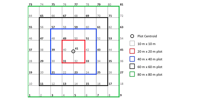
Currently, only the plot is geolocated, the data being contained in vst_perplotperyear.csv columns decimalLatitude and decimalLongitude.
The location of each individual stem is defined in vst_mappingandtagging.csv.
A number of variables are involved, including:
-
pointIDwhich identifies a point on a 10m cell grid centred arounddecimalLatitudeanddecimalLongitude -
stemDistanceandstemAzimuthwhich define the location of a stem, relative to the location ofpointID. The full method used to locate individual stems is detailed indata-raw/wood-survey-data-master/methods/NEON_vegStructure_userGuide_vA.pdf.
NEON_vegStructure_userGuide_vA.pdf
So, to geolocate our individuals, we need to join information from vst_perplotperyear.csv and vst_mappingandtagging.csv into our individual tibble.
We use the family of *_join functions in dplyr to merge columns from different tibbles according to values in shared columns.
Join Basics
There are a number of joins we can perform with dplyr.
Let’s have a look at a few of them with a simple example using some dplyr in-built data:
band_members# A tibble: 3 × 2
name band
<chr> <chr>
1 Mick Stones
2 John Beatles
3 Paul Beatlesband_instruments# A tibble: 3 × 2
name plays
<chr> <chr>
1 John guitar
2 Paul bass
3 Keith guitarThe only variable shared between the two tables is name so this is the only variable we can perform joins over. By default, any *_join function will try to merge on the values of any matched columns in the tables being merged.
Inner joins
band_members %>% inner_join(band_instruments)Joining with `by = join_by(name)`# A tibble: 2 × 3
name band plays
<chr> <chr> <chr>
1 John Beatles guitar
2 Paul Beatles bass inner_join has merged all three unique columns across the two tables into a single tibble. It has only kept the rows in which name values had a match in both tables. In this case only data about John and Paul was contained in both tables.
Left joins
band_members %>% left_join(band_instruments)Joining with `by = join_by(name)`# A tibble: 3 × 3
name band plays
<chr> <chr> <chr>
1 Mick Stones <NA>
2 John Beatles guitar
3 Paul Beatles bass left_join joins on the names in the left hand table and appends any rows from the right hand table in which values in name match. In this case, there is no data for Keith in band_members so he is ignored completely. There is also no match for Mick in band_instruments so NA is returned for plays instead.
Right joins
band_members %>% right_join(band_instruments)Joining with `by = join_by(name)`# A tibble: 3 × 3
name band plays
<chr> <chr> <chr>
1 John Beatles guitar
2 Paul Beatles bass
3 Keith <NA> guitarright_join on the other hand joins on the name in the right hand table. In this case, Mick is dropped completely Keith gets NA for band.
band_members %>% full_join(band_instruments)Joining with `by = join_by(name)`# A tibble: 4 × 3
name band plays
<chr> <chr> <chr>
1 Mick Stones <NA>
2 John Beatles guitar
3 Paul Beatles bass
4 Keith <NA> guitarFinally, a full_join joins on all unique values of name found across the two tables, returning NA where there are no matches between the two tables.
Joining our tables with dplyr
Join vst_mappingandtagging.csv data
Let’s start by merging data from vst_mappingandtagging.csv. Let’s read the data in.
This data set contains taxonomic and within-plot location metadata on individuals collected during mapping and tagging. There is one row per individual in the data set.
names(maptag)[1] "uid" "eventID" "pointID" "stemDistance"
[5] "stemAzimuth" "individualID" "taxonID" "scientificName"
[9] "taxonRank" Let’s see how many matches in column names we have between the two datasets
Challenge: Finding column name matches in two tables
Default left_join
Because we want to match the rest of the tables to our individual data, we use left_join() and supply individual as the first argument and maptag as the second.
individual %>%
  dplyr::left_join(maptag)
Joining with `by = join_by(uid, eventID, individualID)`# A tibble: 14,961 × 18
uid namedLocation date eventID domainID siteID plotID individualID
<chr> <chr> <date> <chr> <chr> <chr> <chr> <chr>
1 a36a162… BART_037.bas… 2015-08-26 vst_BA… D01 BART BART_… NEON.PLA.D0…
2 68dc7ad… BART_037.bas… 2015-08-26 vst_BA… D01 BART BART_… NEON.PLA.D0…
3 a8951ab… BART_044.bas… 2015-08-26 vst_BA… D01 BART BART_… NEON.PLA.D0…
4 eb348ea… BART_044.bas… 2015-08-26 vst_BA… D01 BART BART_… NEON.PLA.D0…
5 2a4478e… BART_044.bas… 2015-08-26 vst_BA… D01 BART BART_… NEON.PLA.D0…
6 e485203… BART_044.bas… 2015-08-26 vst_BA… D01 BART BART_… NEON.PLA.D0…
7 280c904… BART_044.bas… 2015-08-26 vst_BA… D01 BART BART_… NEON.PLA.D0…
8 0e5060e… BART_044.bas… 2015-08-26 vst_BA… D01 BART BART_… NEON.PLA.D0…
9 4918cac… BART_044.bas… 2015-08-26 vst_BA… D01 BART BART_… NEON.PLA.D0…
10 ef16cb9… BART_044.bas… 2015-08-26 vst_BA… D01 BART BART_… NEON.PLA.D0…
# ℹ 14,951 more rows
# ℹ 10 more variables: growthForm <chr>, stemDiameter <dbl>,
# measurementHeight <dbl>, height <dbl>, pointID <dbl>, stemDistance <dbl>,
# stemAzimuth <dbl>, taxonID <chr>, scientificName <chr>, taxonRank <chr>Great we have a merge!
Looks successful right? How do we really know nothing has gone wrong though?
Remember, to successfully merge the tables, the values in the columns the tables are being joined on need to have corresponding values across all join columns to be linked successfully, otherwise it will return NAs. So, although our code ran successfully, it may well not have found any matching rows in maptag to merge into individual.
To check whether things have worked, we can start with inspecting the output for the columns of interest, in this case the maptag columns we are trying to join into individual.
When working interactively and testing out pipes, you can pipe objects into View() for quick inspection. If you provide a character string as an argument, it is used as a name for the data view tab it launches
Clearly this has not worked! We need to start digging into why but we don’t want to have to keep manually checking whether it worked or not. Enter DEFENSIVE PROGRAMMING.
Defensive programming with data
As I mentioned in the Data Management Basics slides, assertr is a useful package for including validation checks in our data pipelines.
In our case, we can use assertr function assert to check that certain columns of interest (stemDistance, stemAzimuth, pointID) are joined successfully (i.e. they contain no NA values).
Note that this only works because I know for a fact that there is data available for all individuals. There may be situations in which NAs are valid missing data, in which case this would not be an appropriate test.
Let’s introduce this check into our pipeline:
individual %>%
  dplyr::left_join(maptag) %>%
  assertr::assert(assertr::not_na, stemDistance, stemAzimuth, pointID)
Joining with `by = join_by(uid, eventID, individualID)`Column 'stemDistance' violates assertion 'not_na' 14961 times
verb redux_fn predicate column index value
1 assert NA not_na stemDistance 1 NA
2 assert NA not_na stemDistance 2 NA
3 assert NA not_na stemDistance 3 NA
4 assert NA not_na stemDistance 4 NA
5 assert NA not_na stemDistance 5 NA
[omitted 14956 rows]
Column 'stemAzimuth' violates assertion 'not_na' 14961 times
verb redux_fn predicate column index value
1 assert NA not_na stemAzimuth 1 NA
2 assert NA not_na stemAzimuth 2 NA
3 assert NA not_na stemAzimuth 3 NA
4 assert NA not_na stemAzimuth 4 NA
5 assert NA not_na stemAzimuth 5 NA
[omitted 14956 rows]
Column 'pointID' violates assertion 'not_na' 14961 times
verb redux_fn predicate column index value
1 assert NA not_na pointID 1 NA
2 assert NA not_na pointID 2 NA
3 assert NA not_na pointID 3 NA
4 assert NA not_na pointID 4 NA
5 assert NA not_na pointID 5 NA
[omitted 14956 rows]Error: assertr stopped executionThe assertr::assert function applies the predicate assertr::not_na on columns stemDistance, stemAzimuth, pointID which checks that each column does not contain NA values.
By appending it onto our pipeline, the function will through an error if the predicate assertion returns FALSE in any of the columns stemDistance, stemAzimuth, pointID. If the assertion is TRUE, the pipeline will continue as expected.
By including this check, I don’t have to guess or manually check whether the merge has been successful. The code will just error if it hasn’t 🙌.
Join vst_perplotperyear.csv
Now let’s carry on and join the perplot data.
First let’s read it in and have a look at the data.
perplot <- readr::read_csv(
  fs::path(raw_data_path, "vst_perplotperyear.csv"),
  show_col_types = FALSE)

perplot
# A tibble: 184 × 13
uid plotID plotType nlcdClass decimalLatitude decimalLongitude
<chr> <chr> <chr> <chr> <dbl> <dbl>
1 93ee1436-cdd8-40b… BART_… distrib… deciduou… 44.0 -71.3
2 4b5f972f-d00f-476… BART_… distrib… deciduou… 44.1 -71.3
3 66594b70-4db4-400… BART_… distrib… deciduou… 44.1 -71.3
4 730098e8-30a7-4b7… BART_… distrib… mixedFor… 44.0 -71.3
5 07c96abe-6d78-481… BART_… distrib… deciduou… 44.1 -71.3
6 557410ec-351d-434… BART_… distrib… mixedFor… 44.1 -71.3
7 afc50622-9684-4d6… BART_… distrib… deciduou… 44.0 -71.3
8 6d597101-9c98-4ba… BART_… distrib… deciduou… 44.0 -71.3
9 591a2808-5add-407… BART_… distrib… mixedFor… 44.0 -71.3
10 12dbf09b-5f23-4ab… BART_… distrib… mixedFor… 44.1 -71.3
# ℹ 174 more rows
# ℹ 7 more variables: geodeticDatum <chr>, easting <dbl>, northing <dbl>,
# utmZone <chr>, elevation <dbl>, elevationUncertainty <dbl>, eventID <chr>Similarly to maptag, we want to exclude eventID and suffix the uid column. This time, however, we will be joining by plotID**
Let’s also move our validation test to the end and add additional columns from perplot we want to check to it, i.e. stemDistance, stemAzimuth, pointID.
perplot <- perplot %>% select(-eventID)

individual %>%
  dplyr::left_join(maptag,
    by = "individualID",
    suffix = c("", "_map")
  ) %>%
  dplyr::left_join(perplot,
    by = c("plotID"),
    suffix = c("", "_ppl")
  ) %>%
  assertr::assert(
    assertr::not_na, decimalLatitude,
    decimalLongitude, plotID, stemDistance, stemAzimuth, pointID
  )
# A tibble: 14,961 × 30
uid namedLocation date eventID domainID siteID plotID individualID
<chr> <chr> <date> <chr> <chr> <chr> <chr> <chr>
1 a36a162… BART_037.bas… 2015-08-26 vst_BA… D01 BART BART_… NEON.PLA.D0…
2 68dc7ad… BART_037.bas… 2015-08-26 vst_BA… D01 BART BART_… NEON.PLA.D0…
3 a8951ab… BART_044.bas… 2015-08-26 vst_BA… D01 BART BART_… NEON.PLA.D0…
4 eb348ea… BART_044.bas… 2015-08-26 vst_BA… D01 BART BART_… NEON.PLA.D0…
5 2a4478e… BART_044.bas… 2015-08-26 vst_BA… D01 BART BART_… NEON.PLA.D0…
6 e485203… BART_044.bas… 2015-08-26 vst_BA… D01 BART BART_… NEON.PLA.D0…
7 280c904… BART_044.bas… 2015-08-26 vst_BA… D01 BART BART_… NEON.PLA.D0…
8 0e5060e… BART_044.bas… 2015-08-26 vst_BA… D01 BART BART_… NEON.PLA.D0…
9 4918cac… BART_044.bas… 2015-08-26 vst_BA… D01 BART BART_… NEON.PLA.D0…
10 ef16cb9… BART_044.bas… 2015-08-26 vst_BA… D01 BART BART_… NEON.PLA.D0…
# ℹ 14,951 more rows
# ℹ 22 more variables: growthForm <chr>, stemDiameter <dbl>,
# measurementHeight <dbl>, height <dbl>, uid_map <chr>, pointID <dbl>,
# stemDistance <dbl>, stemAzimuth <dbl>, taxonID <chr>, scientificName <chr>,
# taxonRank <chr>, uid_ppl <chr>, plotType <chr>, nlcdClass <chr>,
# decimalLatitude <dbl>, decimalLongitude <dbl>, geodeticDatum <chr>,
# easting <dbl>, northing <dbl>, utmZone <chr>, elevation <dbl>, …Awesome!! It’s worked! 🎉
Using the assignment pipe
Now that we are happy with our data we can use a new operator, the assignment pipe (%<>%).
This allows us to both pipe an object forward into an expression and also update it with the resulting value.
Note that this operator can have unexpected results if you run the same code multiple times in an interactive session. Use it in scripts that will be run from top to bottom only once.
Update individual.R
Let’s update our individual.R script again with the additional code we’ve just written for reading in and merging the maptag and perplot data.
Add the following code and comments to individual.R:
# Combine NEON data tables ----
# read in additional tables
maptag <- readr::read_csv(
  fs::path(
    raw_data_path,
    "vst_mappingandtagging.csv"
  ),
  show_col_types = FALSE
) %>%
  select(-eventID)

perplot <- readr::read_csv(
  fs::path(
    raw_data_path,
    "vst_perplotperyear.csv"
  ),
  show_col_types = FALSE
) %>%
  select(-eventID)

# Left join tables to individual
individual %<>%
  left_join(maptag,
    by = "individualID",
    suffix = c("", "_map")
  ) %>%
  left_join(perplot,
    by = "plotID",
    suffix = c("", "_ppl")
  ) %>%
  assertr::assert(
    assertr::not_na, stemDistance, stemAzimuth, pointID,
    decimalLongitude, decimalLatitude, plotID
  )
We can now move on to geolocate our individuals!