Front Matter & Markdown Basics
Creating a Scientific Report
In this part of the course, we will use Quarto to create a reproducible presentation document for our analysis, combining our code and it’s output with text in the form of markdown!
Create your first .qmd!
Create new .qmd file
Let’s start by creating a new .qmd file in RStudio.
File > New File > Quarto Document… > Document
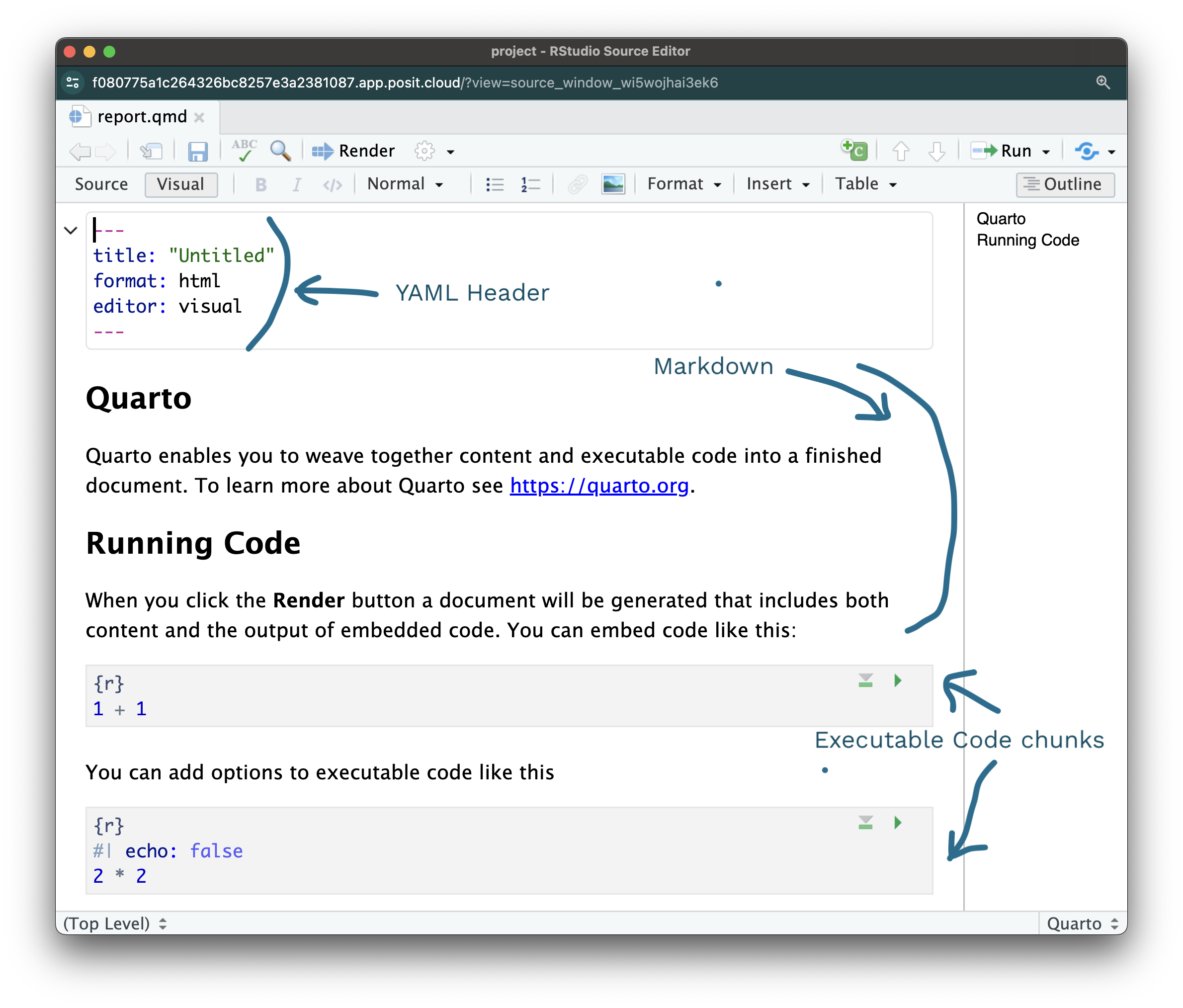
The new document default content demonstrates the 3 main elements that make up a Quarto document:
- At the top, the YAML header where we specify front matter metadata about the document.
- The main body of the document where we write our text in markdown.
- The code chunks where we write our executable R code.
Save as report.qmd
Let’s save the file as report.qmd in the root of our project directory.
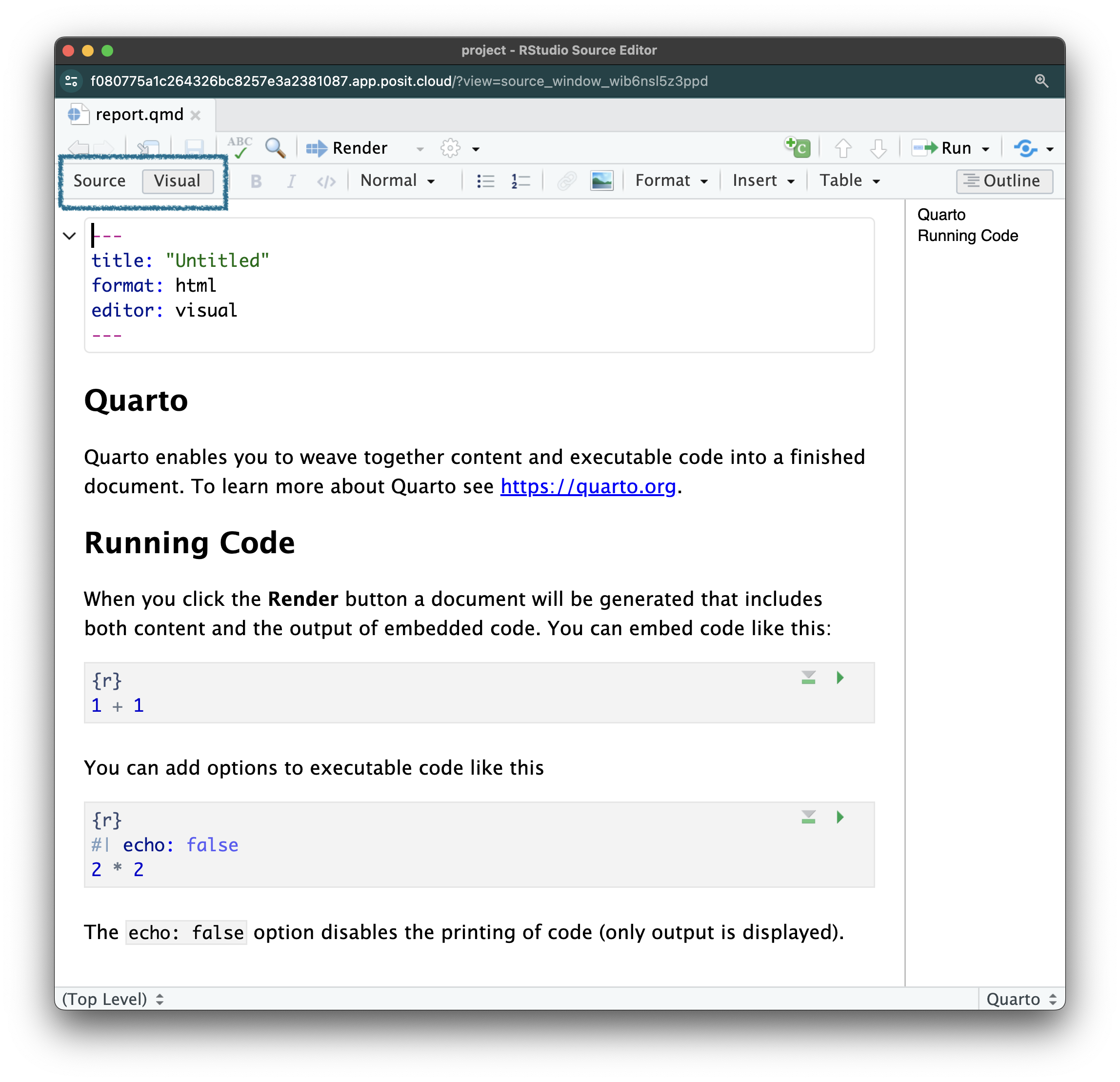
Quarto Editing Modes
Quarto documents can be edited in two modes: Source and Visual.
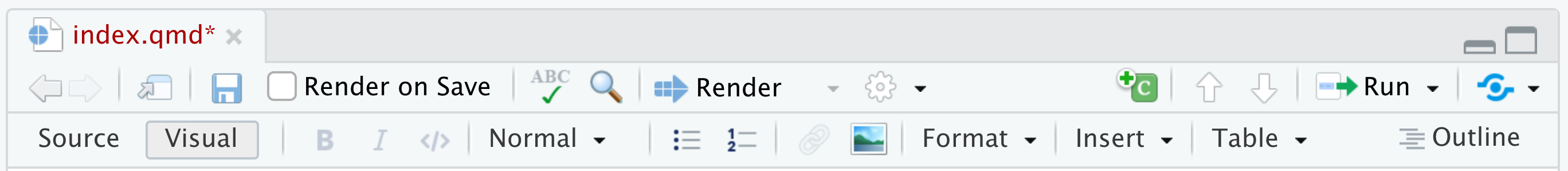
To switch between the two modes, you can use the buttons in the top left of the editor.
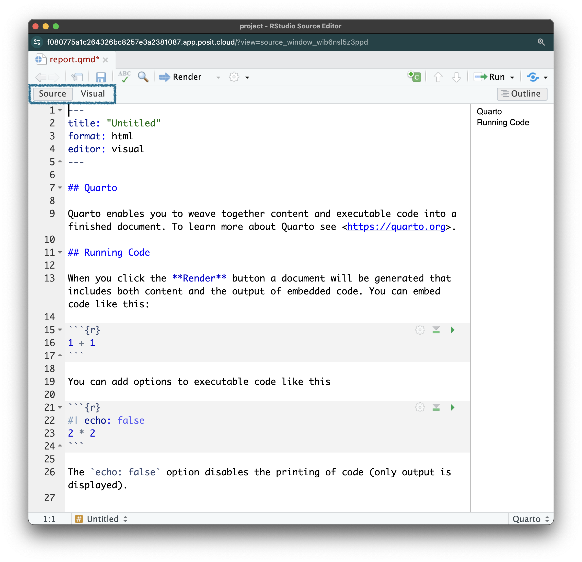
Source Vs Visual Editing
The Quarto Visual Editor is a WhatYouSeeIsWhatYouGet editor that allows you to edit your document in a more visual way and is normally the mode launched by default in Rstudio.
Find out more about the Visual Editor.
The Source editor is a text editor that allows you to edit the raw markdown and code that makes up your document. It is more stable and is the mode we will be using more often for this course.
Render report.qmd
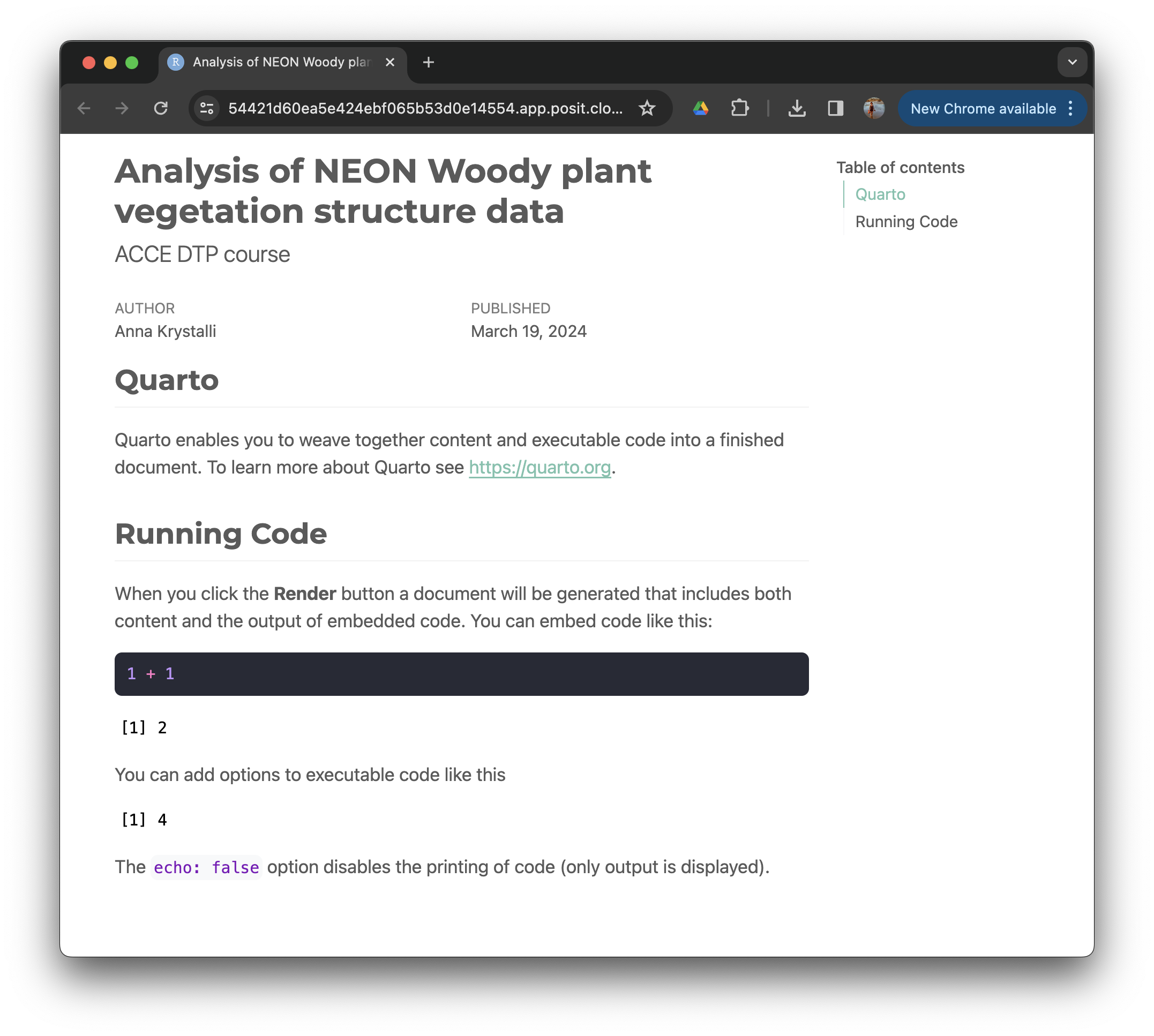
Render the document by clicking on the Render button.

Quarto will the Knit the document by running all the computations and rendering any markdown to an .html document:
Edit Front matter YAML header
The yaml header contains metadata about the document.
It is contained between the --- separators at the top of the file and is encoded as YAML, a human friendly data serialization standard for all programming languages.
The key thing to know about YAML is that indentation is extremely important!. So make sure you copy any example YAML code exactly, ensuring correct indentation. If you get errors, check your indentation.
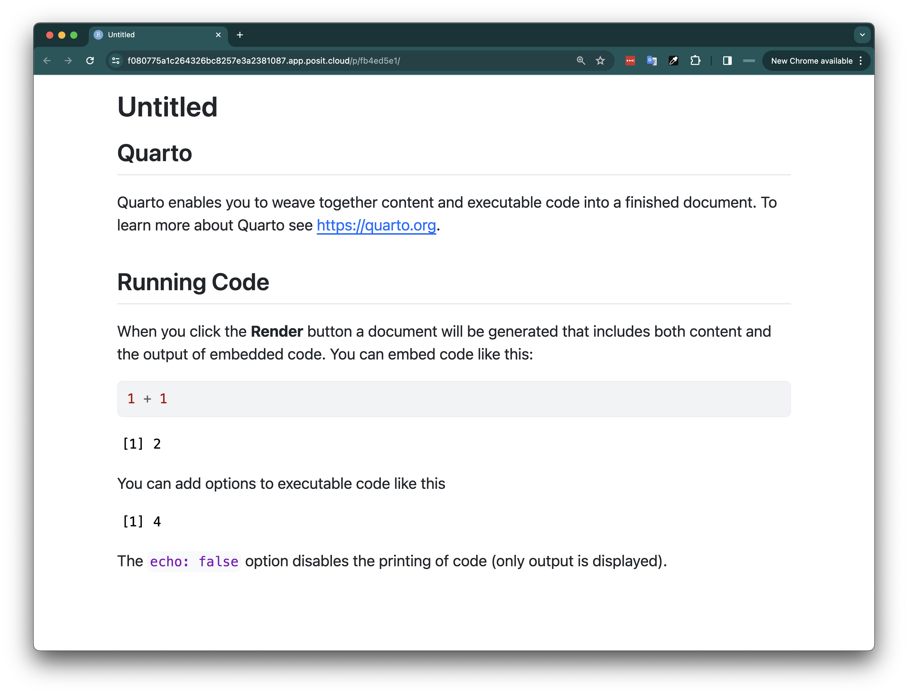
The default YAML header contains the following metadata:
---
title: "Untitled"
format: html
editor: visual
----
title: A field to specify a title of the document. -
format: The format of the document. We will be using the defaulthtmlfor this course. -
editor: The default editor mode the document will be opened with.
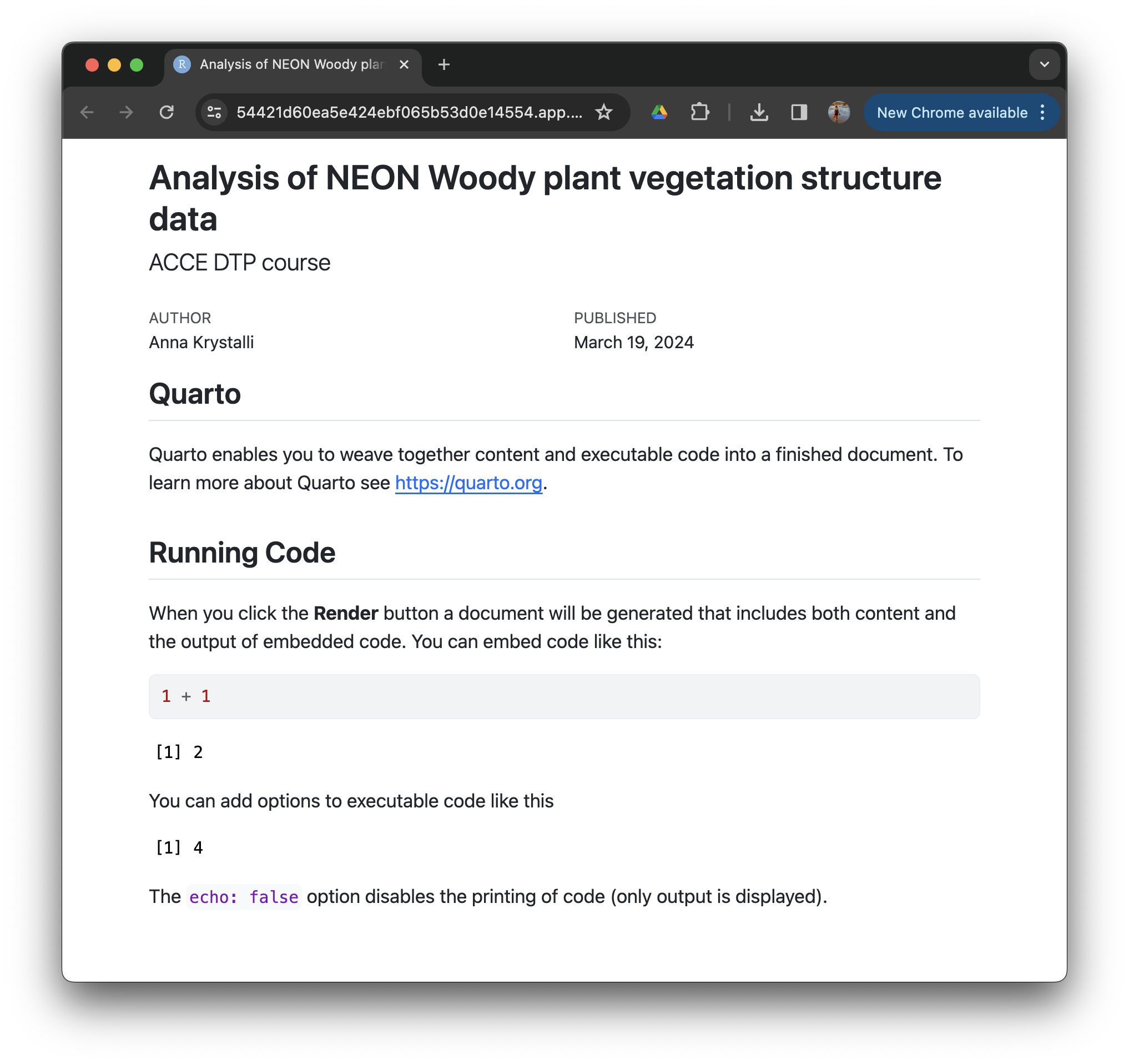
Let’s go ahead and update the title and add some more metadata to the header.
---
title: "Analysis of NEON Woody plant vegetation structure data"
subtitle: "ACCE DTP course"
author: "Anna Krystalli"
date: "2024-03-19"
format: html
editor: visual
---
Let’s re-render and have a look at our updated document:
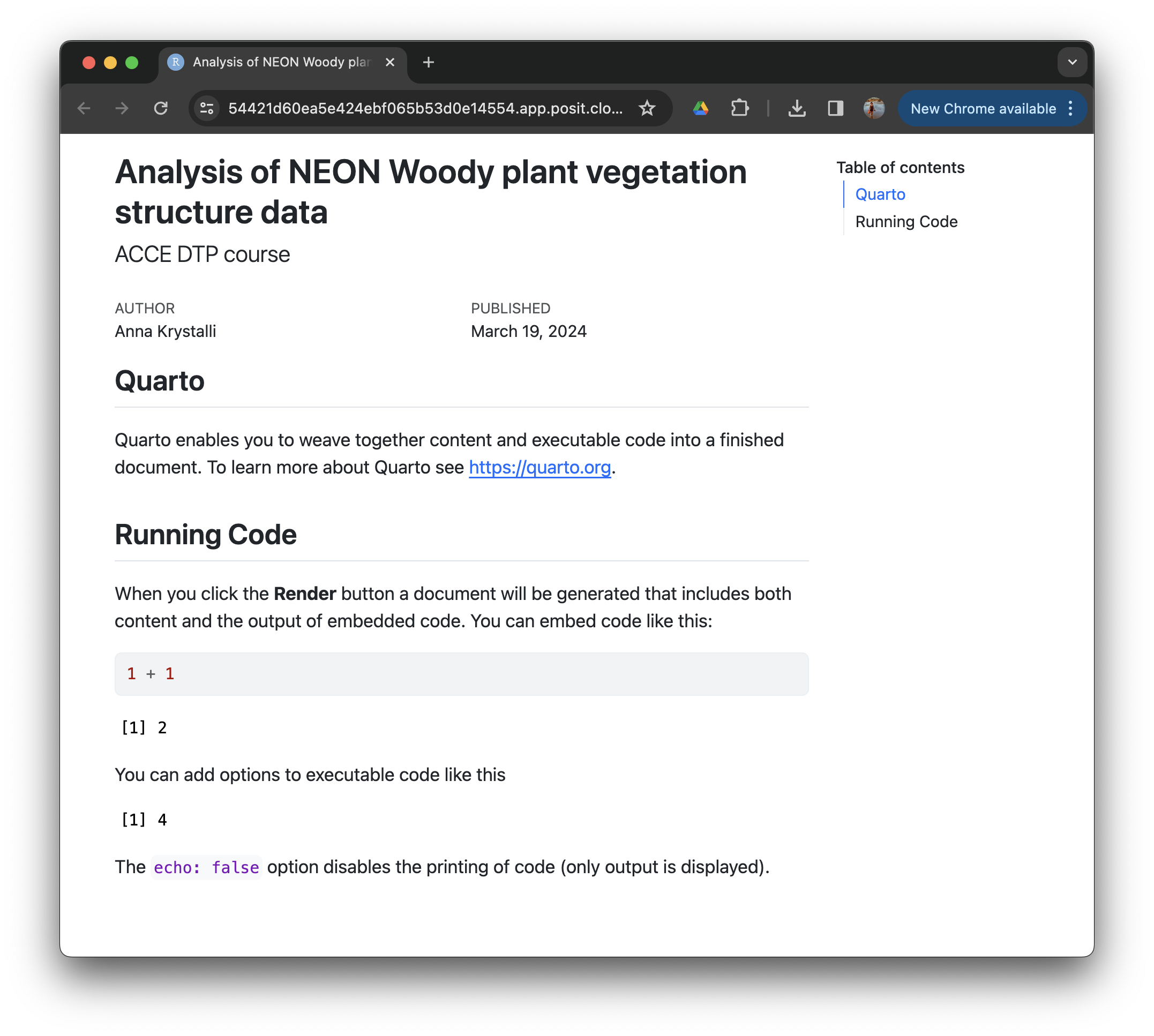
Add a floating table of contents
We can add a table of contents (TOC) using the toc option and specify a floating toc using the toc_float option. For example:
---
title: "Analysis of NEON Woody plant vegetation structure data"
subtitle: "ACCE DTP course"
author: "Anna Krystalli"
date: "2024-03-19"
format:
  html:
    toc: true
editor: visual
---
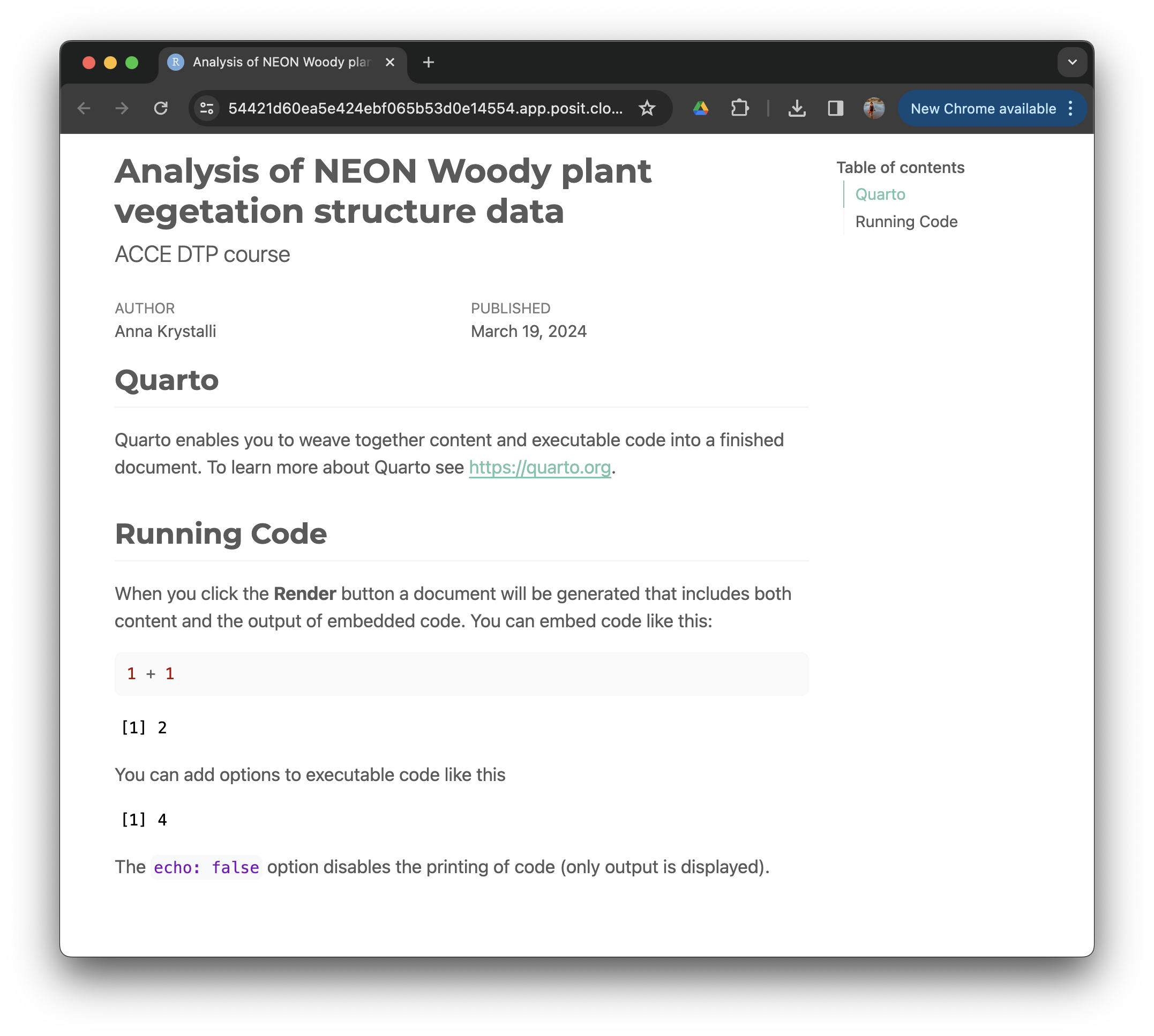
Choose a theme
There are several options that control the appearance of HTML documents:
-
themespecifies the Bootstrap theme to use for the page (themes are drawn from the Bootswatch theme library). Valid themes includedefault,bootstrap,cerulean,cosmo,darkly,flatly,journal,lumen,paper,readable,sandstone,simplex,spacelab,united, andyeti.
I’m going to go ahead and choose the minty theme but feel free to experiment and choose a theme that you like.
---
title: "Analysis of NEON Woody plant vegetation structure data"
subtitle: "ACCE DTP course"
author: "Anna Krystalli"
date: "2024-03-19"
format:
  html:
    toc: true
    theme: minty
editor: visual
---
Once rendered, my theme of choice looks like this:
Choose code highlights
Field highlight-style specifies the code syntax highlighting style.
Supported styles include default, tango, pygments, kate, monochrome, espresso, zenburn, haddock, breezedark, and textmate as well as a bunch of new styles which can be found here:
I’m picking one of the extended themes called dracula!
---
title: "Analysis of NEON Woody plant vegetation structure data"
subtitle: "ACCE DTP course"
author: "Anna Krystalli"
date: "2024-03-19"
format:
  html:
    toc: true
    theme: minty
    highlight-style: dracula
editor: visual
---
Before moving on to adding content to our document, let’s have a look at some Markdown basics.
Markdown basics
The text in an Quarto document is written with the Markdown syntax. Precisely speaking, it is Pandoc’s Markdown.
We use a small number of notations to markup our text with some common html tags
Text
normal textnormal text
*italic text*italic text
**bold text**bold text
***bold italic text***bold italic text
superscript^2^superscript2
~~strikethrough~~strikethrough
Headers
markdown
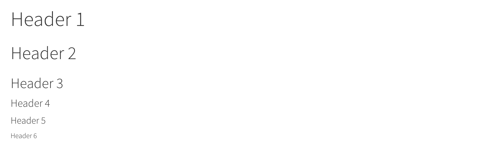
# Header 1
## Header 2
### Header 3
#### Header 4
##### Header 5
###### Header 6
rendered html
Unordered lists
markdown
- first item in the list
- second item in list
- third item in list
rendered html
- first item in the list
- second item in list
- third item in list
Ordered lists
markdown
1. first item in the list
1. second item in list
1. third item in list
rendered html
- first item in the list
- second item in list
- third item in list
Blockquotes
markdown
> this text will be quotedrendered html
this text will be quoted
Code
Annotate code inline
markdown
`this text will appear as code` inlinerendered html
this text will appear as code inline
Evaluate r code inline
a <- 10markdown
the value of parameter *a* is `{r} a`rendered html
the value of parameter a is 10
Images
Provide either a path to a local image file or the URL of an image.
markdown
rendered html

Basic tables in markdown
markdown
    Table Header  | Second Header
                - | -
    Cell 1        | Cell 2
    Cell 3        | Cell 4
rendered html
| Table Header | Second Header |
|---|---|
| Cell 1 | Cell 2 |
| Cell 3 | Cell 4 |
Check out handy online .md table converter
Hyperlinks
markdown
[Download R](http://www.r-project.org/)
[RStudio](http://www.rstudio.com/)Mathematical expressions
Quarto supports mathematical notations through MathJax.
You can write LaTeX math expressions inside a pair of dollar signs, e.g. $\alpha+\beta$ renders \(\alpha+\beta\). You can use the display style with double dollar signs:
$$\bar{X}=\frac{1}{n}\sum_{i=1}^nX_i$$\[\bar{X}=\frac{1}{n}\sum_{i=1}^nX_i\]
Visual Editor
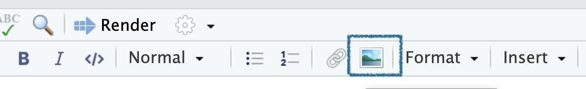
Much of the markdown syntax can be added to documents via the visual editor.
The editor toolbar includes buttons for the most commonly used formatting commands, e.g:
- Formatting text to appear as bold, italic, or code
- Creating headers
- Creating lists
Format
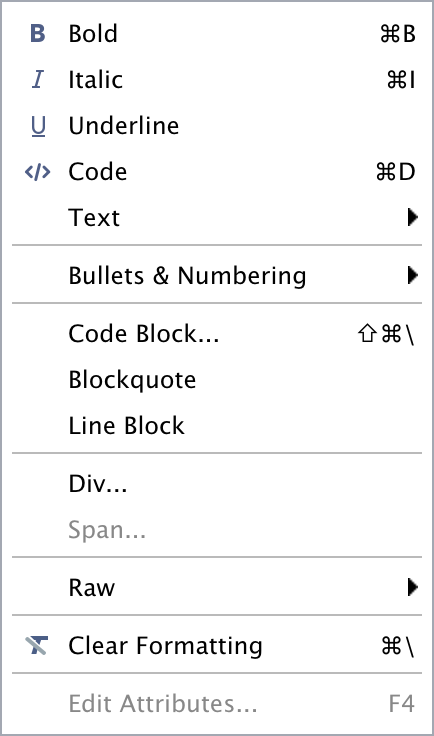
Insert 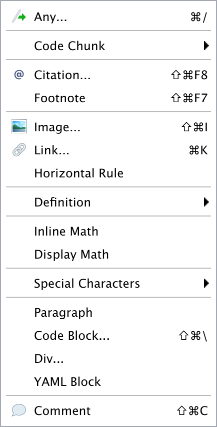
Table 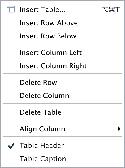
Add images with the Visual Editor
To add an image via the visual editor, click on the picture button in the toolbar.
This opens up a file dialog box where you can select the image you want to insert by clicking on Browse….
You can also add a add a caption and a link to the image
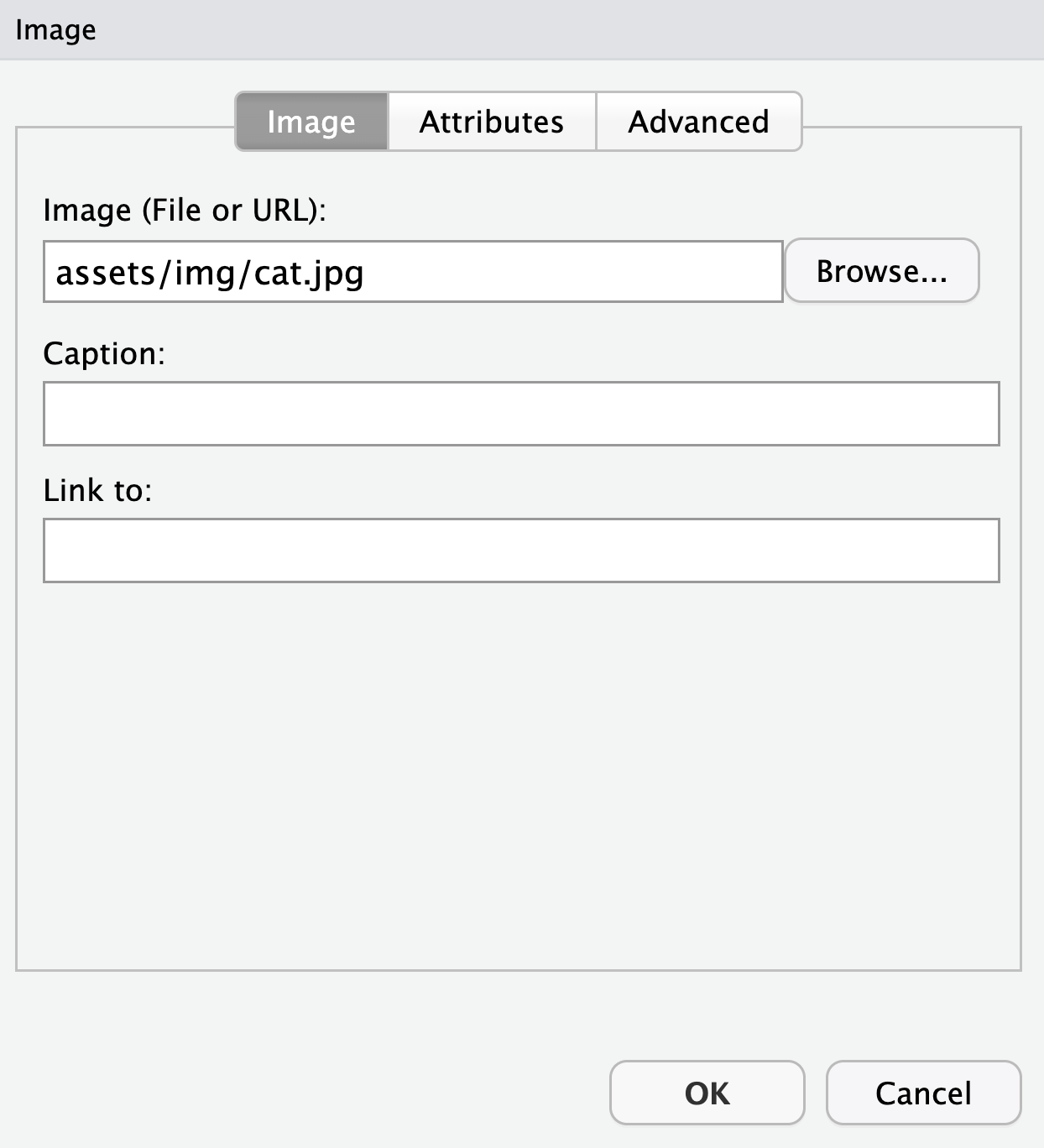 Click OK and the image is now inserted.
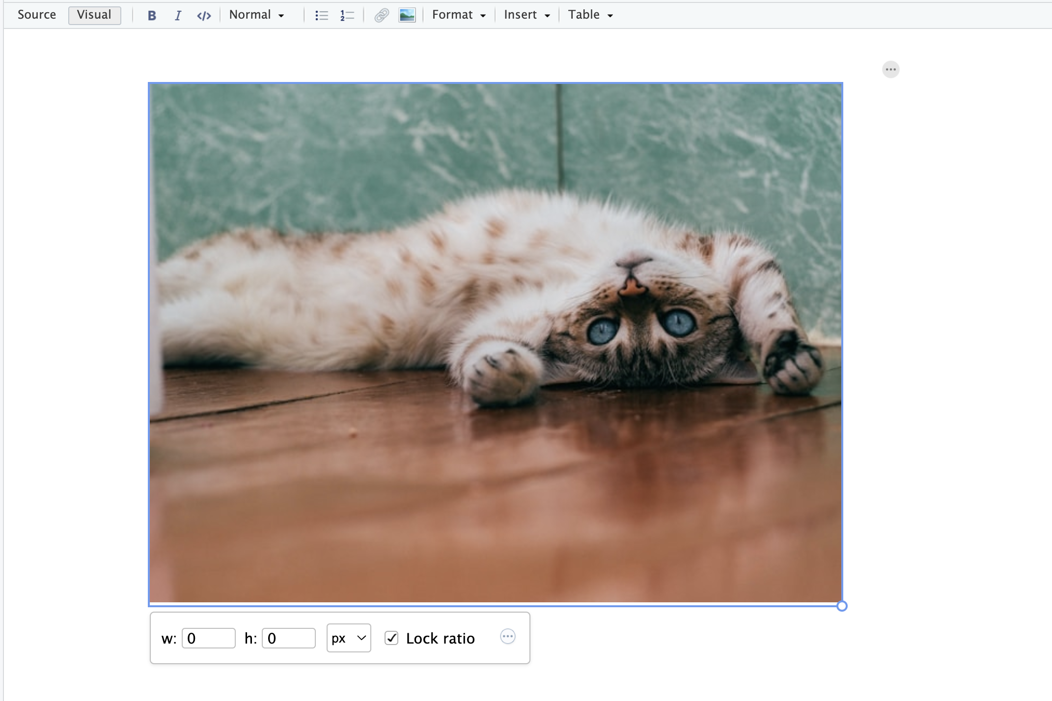
Resize images with Visual Editor
The Visual editor allows to resize images via the user interface.
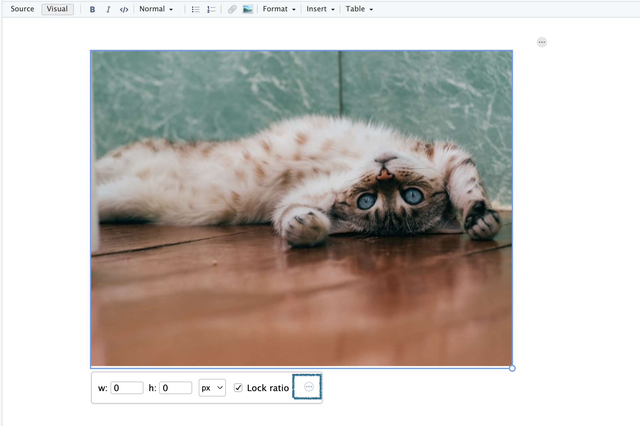
To change any attributes of an image, click on the round ... button in the image toolbar.
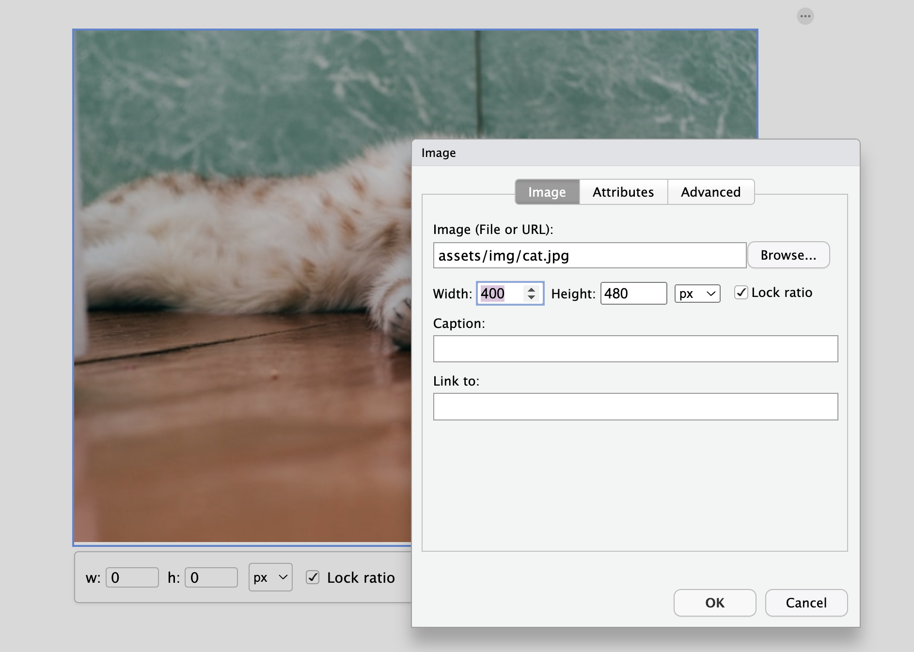
This opens up a image dialog box where you can change the image size, alignment and more.
You can reduce the size by editing the width and or height fields.
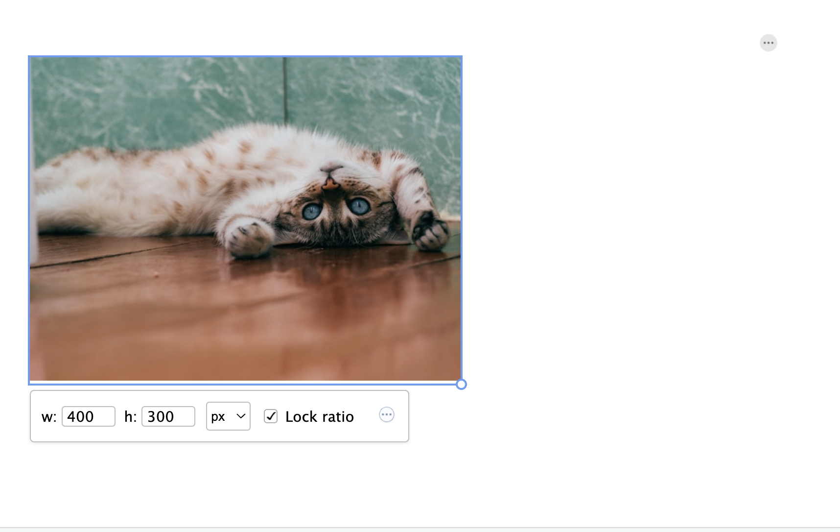
Click ok and the image is now resized.
Edit Content
Next let’s start adding content related to our analysis.
To do so, let’s first remove all the default content in the document EXCEPT FOR THE YAML HEADER and start with a clean slate.
TASK: Create a "Background" section using headers
Create a
BackgroundHeader: Create a new level 2 header section called"Background"using the appropriate number of the#symbol followed by the header text.-
Write a short description of the data set and analysis: Write a short description of the NEON Vegetation structure dataset and the objective of the analysis.
Have a look at the project README in
data-raw/wood-survey-data-masterwhich contains some useful information you might be able to copy. _Note: You’ll likely need to switch to the Source editor to paste raw markdown_ -
Make use of markdown annotation to:
- highlight important information
- include links to sources or further information. The NEON Data Portal Vegetation Structure URL might come in handy here: https://data.neonscience.org/data-products/DP1.10098.001
-
Add an image related to the data.
- perhaps a logo or a relevant image to the organisms in question (see
data-raw/wood-survey-data-masterfor a NEON logo). - have a look online, especially on sites like unsplash that offer free to use images. Note: To upload images to your project, use the Upload files to server button in the File pane on the bottom right of Posit Cloud interface.
- include the source underneath for attribution.
- see if you can resize it.
- perhaps a logo or a relevant image to the organisms in question (see
-
Include a brief data preparation section:
- Use a list to describe a couple of steps in our data preparation process.
- Mention the script that contains the data preparation code.
---
title: "Analysis of NEON Woody plant vegetation structure data"
subtitle: "ACCE DTP course"
author: "Anna Krystalli"
date: "2024-03-19"
format:
html:
toc: true
theme: minty
highlight-style: dracula
editor: visual
---
## Background
{width="200"}
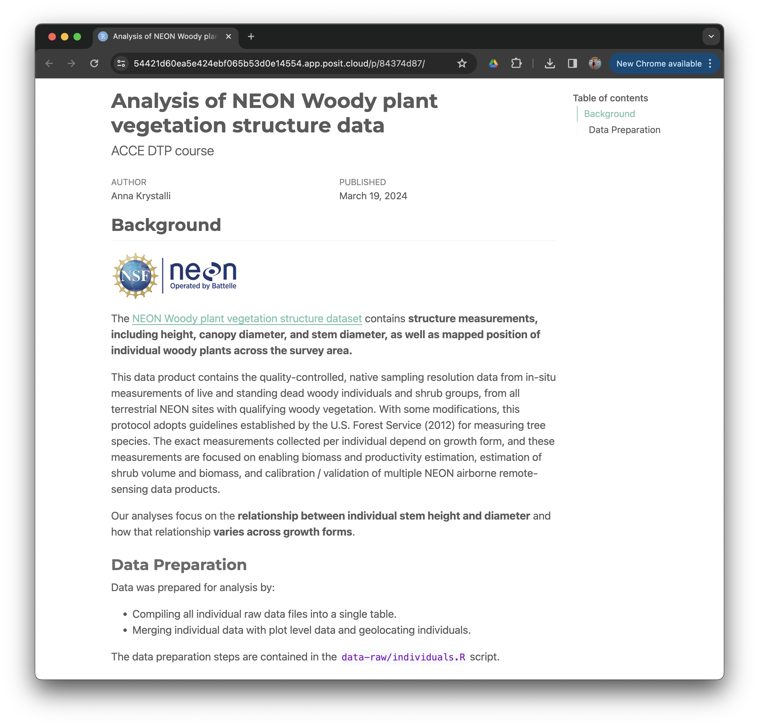
The [NEON Woody plant vegetation structure dataset](https://data.neonscience.org/data-products/DP1.10098.001) contains **structure measurements, including height, canopy diameter, and stem diameter, as well as mapped position of individual woody plants across the survey area.**
This data product contains the quality-controlled, native sampling resolution data from in-situ measurements of live and standing dead woody individuals and shrub groups, from all terrestrial NEON sites with qualifying woody vegetation. With some modifications, this protocol adopts guidelines established by the U.S. Forest Service (2012) for measuring tree species. The exact measurements collected per individual depend on growth form, and these measurements are focused on enabling biomass and productivity estimation, estimation of shrub volume and biomass, and calibration / validation of multiple NEON airborne remote-sensing data products.
Our analyses focus on the **relationship between individual stem height and diameter** and how that relationship **varies across growth forms**.
### Data Preparation
Data was prepared for analysis by:
- Compiling all individual raw data files into a single table.
- Merging individual data with plot level data and geolocating individuals.
The data preparation steps are contained in the `data-raw/individuals.R` script.