```{r}
print('hello world!')
```
[1] "hello world!"![]()
Creating a Scientific Report
R code blocks execute code.
Code blocks that use braces around the language name (e.g. ```{r}) are executable, and will be run by Quarto during render.
They can be used as a means to perform computations, render R output like text, tables, or graphics into documents or to simply display code for illustration without evaluating it.
You can quickly insert an R code block with:
Ctrl + Alt + I (OS X: Cmd + Option + I)```{r} and ```.block notation in .rmd
```{r}
print('hello world!')
```[1] "hello world!"rendered html code and output
print('hello world!')[1] "hello world!"Blocks can be labelled with block names, names must be unique. This can be useful for debugging as well as for referencing blocks within text.
You’ll note that we are using some special comments starting with #| at the top of the code block. These are used to define cell level options, including labels, execution and display options and output cross-referencing
```{r}
#| label: block-name
print('hello world!')
```
[1] "hello world!"There are a wide variety of options available for customizing output from executed code. All of these options can be specified either globally (in the document front-matter -YAML header-) or per code-block.
Block options control how code and outputs are evaluated and presented.
Standard block options include:
| Option | Description |
|---|---|
eval |
Evaluate the code chunk (if false, just echos the code into the output). |
echo |
Include the source code in output |
output |
Include the results of executing the code in the output (true, false, or asis to indicate that the output is raw markdown and should not have any of Quarto’s standard enclosing markdown). |
warning |
Include warnings in the output. |
error |
Include errors in the output (note that this implies that errors executing code will not halt processing of the document). |
include |
Catch all for preventing any output (code or results) from being included (e.g. include: false suppresses all output from the code block). |
echo
block notation in .rmd
```{r}
#| label: hide-code
#| echo: false
print('hello world!')
```
rendered html code and output
[1] "hello world!"eval
block notation in .rmd
```{r}
#| label: dont-eval
#| eval: false
print('hello world!')
```
rendered html code and output
print('hello world!')Let’s move on to start introducing our data and some of the initial summary statistics plots we’ve generated. So we’ll now need to start introducing executable code to our document.
analysis.R setup sectionWe’ll start by adding the top section of our analysis.R script to the report into a setup code chunk.
Let’s include:
the code block that loads the necessary packages,
reads in the data
subsets the data
growth forms the growth form levels
We’ll also use some code options to control the display and output of the code block:
label: setup to label the code block with the name setup
code-fold: true to fold the code block by defaultmessage: false to suppress messages from the code block. This is useful for hiding messages from loading packages and reading in data.Your code chunk should look something like this:
```{r}
#| label: setup
#| code-fold: true
#| message: false
## Setup ----
# Load libraries
library(dplyr)
library(ggplot2)
# Load data
individual <- readr::read_csv(
  here::here("data", "individual.csv")
) %>%
  select(stem_diameter, height, growth_form)

## Subset analysis data ----
analysis_df <- individual %>%
  filter(complete.cases(.), growth_form != "liana")

## Order growth form levels
gf_levels <- table(analysis_df$growth_form) %>%
  sort() %>%
  names()
analysis_df <- analysis_df %>%
  mutate(growth_form = factor(growth_form,
    levels = gf_levels
  ))

```Let’s also add some descriptive text to describe the data that will calculate and report dataset characteristics using inline code.
The final data set contains a total of **`{r} nrow(analysis_df)`**It’s useful for a reader to have an idea of what data they are working with. One way to do this is to just print the contents of our tibble to the report.
Quarto provides additional ways to display data natively. One way is to format printed tibbles into an HTML table with paging for row and column overflow, allowing a user to navigate the entire dataset!
To do this, first we print our dataset in a code block:
```{r}
#| echo: false
#| label: tbl-print
analysis_df
```
Then we add option df-print: paged to the document front matter to set the default display of data frames to paged.
Our document should now look something like this:
---
title: "Analysis of NEON Woody plant vegetation structure data"
subtitle: "ACCE DTP course"
author: "Anna Krystalli"
date: "2024-03-19"
format:
html:
toc: true
theme: minty
highlight-style: dracula
df-print: paged
editor: visual
---
## Background
{width="200"}
The [NEON Woody plant vegetation structure dataset](https://data.neonscience.org/data-products/DP1.10098.001) contains **structure measurements, including height, canopy diameter, and stem diameter, as well as mapped position of individual woody plants across the survey area.**
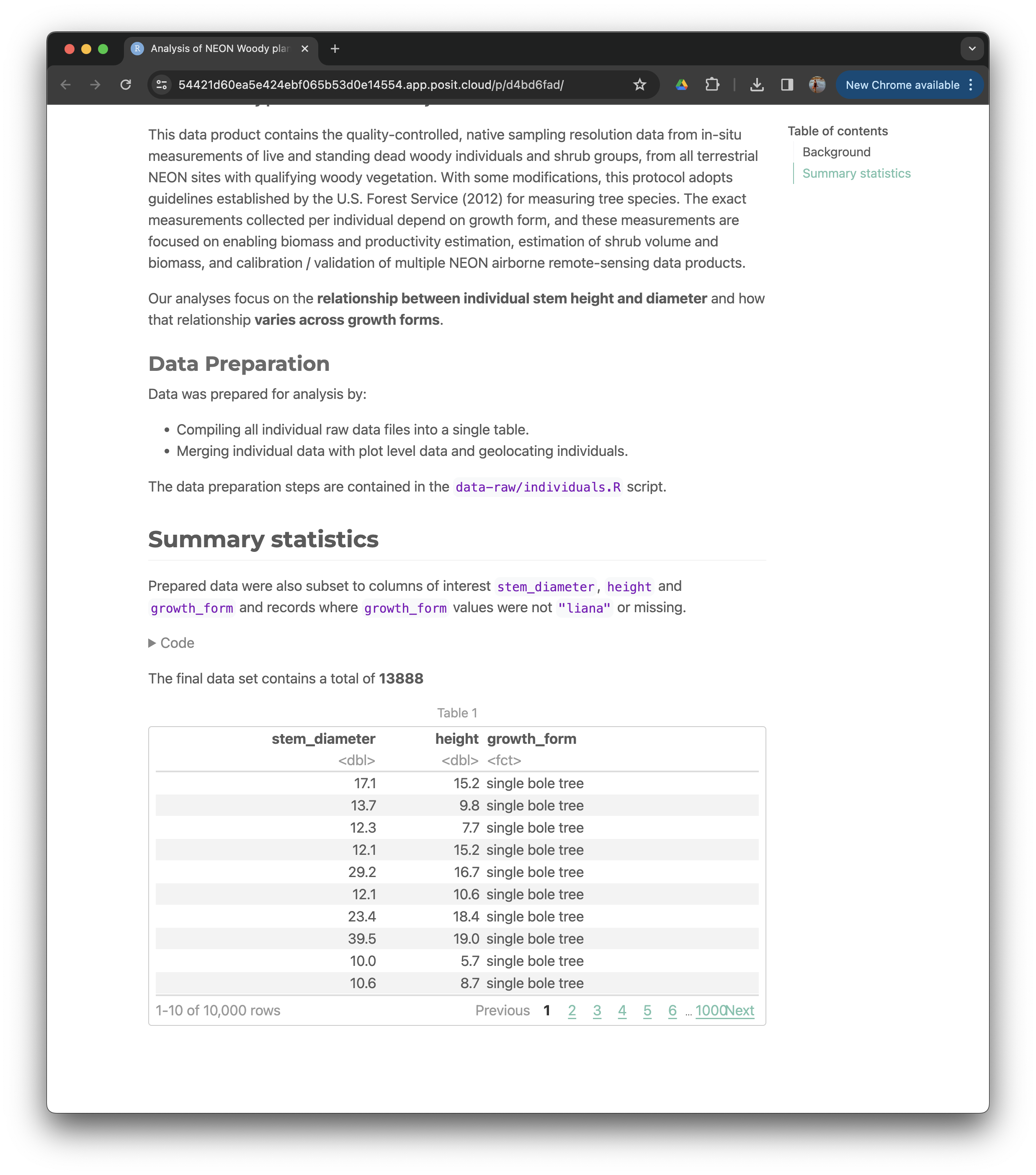
This data product contains the quality-controlled, native sampling resolution data from in-situ measurements of live and standing dead woody individuals and shrub groups, from all terrestrial NEON sites with qualifying woody vegetation. With some modifications, this protocol adopts guidelines established by the U.S. Forest Service (2012) for measuring tree species. The exact measurements collected per individual depend on growth form, and these measurements are focused on enabling biomass and productivity estimation, estimation of shrub volume and biomass, and calibration / validation of multiple NEON airborne remote-sensing data products.
Our analyses focus on the **relationship between individual stem height and diameter** and how that relationship **varies across growth forms**.
### Data Preparation
Data was prepared for analysis by:
- Compiling all individual raw data files into a single table.
- Merging individual data with plot level data and geolocating individuals.
The data preparation steps are contained in the `data-raw/individuals.R` script.
## Summary statistics
Prepared data were also subset to columns of interest `stem_diameter`, `height` and `growth_form` and rows filtered to complete cases. Liana growth forms were removed.
```{r}
#| label: setup
#| code-fold: true
#| message: false
## Setup ----
# Load libraries
library(dplyr)
library(ggplot2)
# Load data
individual <- readr::read_csv(
here::here("data", "individual.csv")
) %>%
select(stem_diameter, height, growth_form)
## Subset analysis data ----
analysis_df <- individual %>%
filter(complete.cases(.), growth_form != "liana")
## Order growth form levels
gf_levels <- table(analysis_df$growth_form) %>%
sort() %>%
names()
analysis_df <- analysis_df %>%
mutate(growth_form = factor(growth_form,
levels = gf_levels
))
```
The final data set contains a total of **11626**
```{r}
#| echo: false
#| label: tbl-print
analysis_df
```And if we render the report, we will see our taxon dataset printed as a paged table.
Let’s now go ahead and add the initial exploratory plots we’ve generated in analysis.R to the report. We’ll also use this opportunity to introduce output cross-referencing.
A really useful feature for Scientific Writing of Quarto is the ability to cross-reference code blocks and their outputs through the use of special labels and referencing notation. See more about cross-referencing.
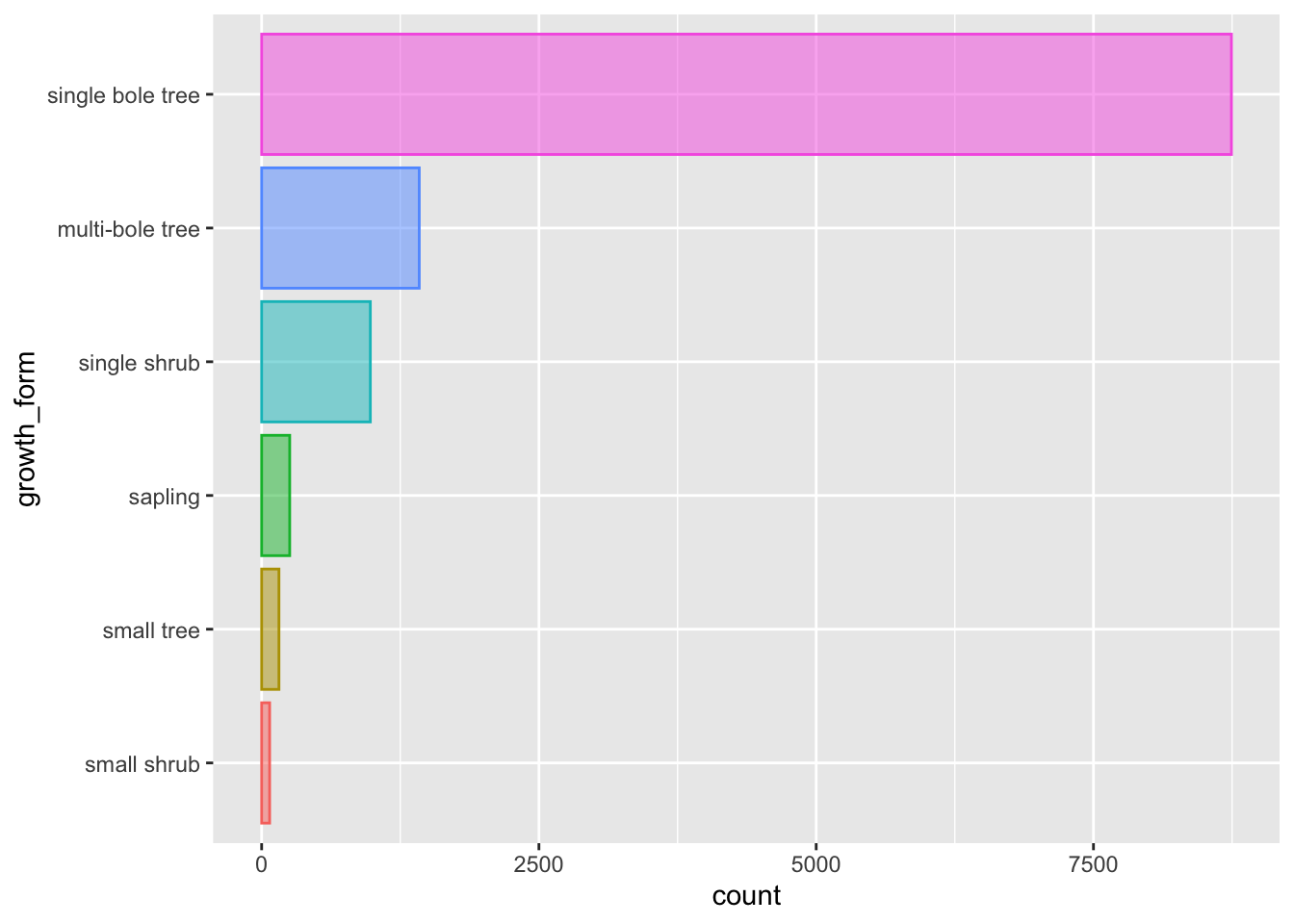
We’ll start by adding a plot of the distribution of sample occurrence counts across growth forms in the dataset.
Let’s add the ggplot code we generated for that plot to the report in a new code block with the folowing code block options:
- echo: false to suppress the code from being displayed in the output.
- label: fig-growth-form-counts to label the code block with the name fig-growth-form-counts. This will allow us to reference the plot in the text but it’s very important to use the prefix fig- in the label name.
- fig-cap: "Distribution of individual counts across growth forms." to add a caption to the plot. This is also necessary for cross referencing the output of the cell.
```{r}
#| echo: false
#| label: fig-growth-form-counts
#| fig-cap: "Distribution of individual counts across growth forms."

analysis_df %>%
  ggplot(aes(
    y = growth_form, colour = growth_form,
    fill = growth_form
  )) +
  geom_bar(alpha = 0.5, show.legend = FALSE)


```
which should render to:
Note how the special label introduces a figure number to the figure caption.
We can use the same label to reference the plot in the text, using the reference notation @. For example, we can then write the following markdown text below the code block:
@fig-growth-form-counts shows the distribution of individual counts across growth forms in the dataset.which renders to the following text:
Figure 1 shows the distribution of individual counts across growth forms in the dataset.
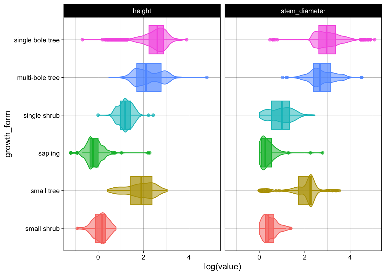
Let’s also add the faceted exploratory plots we generated in analysis.R to the report. These are the violin plots of the log distribution of height and stem_diameter across growth forms.
Let’s add the code for both plots to a new code block with the following code block options:
- echo: false to suppress the code from being displayed in the output.
- label: fig-violin-plots to label the code block with the name fig-violin-plots.
- fig-cap: "Distribution of log stem_diameter and log height across growth forms" to add a caption to the plot.
```{r}
#| echo: false
#| label: fig-violin-plots
#| fig-cap: "Distribution of log stem_diameter and log height across growth forms"
analysis_df %>%
  tidyr::pivot_longer(
    cols = c(stem_diameter, height),
    names_to = "var",
    values_to = "value"
  ) %>%
  ggplot(aes(
    x = log(value), y = growth_form,
    colour = growth_form, fill = growth_form
  )) +
  geom_violin(alpha = 0.5, trim = TRUE, show.legend = FALSE) +
  geom_boxplot(alpha = 0.7, show.legend = FALSE) +
  facet_grid(~var) +
  theme_linedraw()

```
Which should render to:
Again, we can see that Quarto has generated a figure number and the label to reference the plot in the text, so let’s add the following markdown below the code block:
@fig-violin-plots shows the log distribution of stem diameter and log height across growth forms.which will render to:
Figure 2 shows the log distribution of stem diameter and log height across growth forms.
You report should now look a bit like:
---
title: "Analysis of NEON Woody plant vegetation structure data"
subtitle: "ACCE DTP course"
author: "Anna Krystalli"
date: "2024-03-19"
format:
html:
toc: true
theme: minty
highlight-style: dracula
df-print: paged
editor: visual
---
## Background
{width="200"}
The [NEON Woody plant vegetation structure dataset](https://data.neonscience.org/data-products/DP1.10098.001) contains **structure measurements, including height, canopy diameter, and stem diameter, as well as mapped position of individual woody plants across the survey area.**
This data product contains the quality-controlled, native sampling resolution data from in-situ measurements of live and standing dead woody individuals and shrub groups, from all terrestrial NEON sites with qualifying woody vegetation. With some modifications, this protocol adopts guidelines established by the U.S. Forest Service (2012) for measuring tree species. The exact measurements collected per individual depend on growth form, and these measurements are focused on enabling biomass and productivity estimation, estimation of shrub volume and biomass, and calibration / validation of multiple NEON airborne remote-sensing data products.
Our analyses focus on the **relationship between individual stem height and diameter** and how that relationship **varies across growth forms**.
### Data Preparation
Data was prepared for analysis by:
- Compiling all individual raw data files into a single table.
- Merging individual data with plot level data and geolocating individuals.
The data preparation steps are contained in the `data-raw/individuals.R` script.
## Summary statistics
Prepared data were also subset to columns of interest `stem_diameter`, `height` and `growth_form` and records where `growth_form` values were not `"liana"` or missing.
```{r}
#| label: setup
#| code-fold: true
#| message: false
## Setup ----
# Load libraries
library(dplyr)
library(ggplot2)
# Load data
individual <- readr::read_csv(
here::here("data", "individual.csv")
) %>%
select(stem_diameter, height, growth_form)
## Subset analysis data ----
analysis_df <- individual %>%
filter(complete.cases(.), growth_form != "liana")
## Order growth form levels
gf_levels <- table(analysis_df$growth_form) %>%
sort() %>%
names()
analysis_df <- analysis_df %>%
mutate(growth_form = factor(growth_form,
levels = gf_levels
))
```
The final data set contains a total of **11626**
```{r}
#| echo: false
#| label: tbl-print
analysis_df
```
```{r}
#| echo: false
#| label: fig-growth-form-counts
#| fig-cap: "Distribution of individual counts across growth forms."
analysis_df %>%
ggplot(aes(
y = growth_form, colour = growth_form,
fill = growth_form
)) +
geom_bar(alpha = 0.5, show.legend = FALSE)
```
@fig-growth-form-counts shows the distribution of individual counts across growth forms in the dataset.
```{r}
#| echo: false
#| label: fig-violin-plots
#| fig-cap: "Distribution of log stem_diameter and log height across growth forms"
analysis_df %>%
tidyr::pivot_longer(
cols = c(stem_diameter, height),
names_to = "var",
values_to = "value"
) %>%
ggplot(aes(
x = log(value), y = growth_form,
colour = growth_form, fill = growth_form
)) +
geom_violin(alpha = 0.5, trim = TRUE, show.legend = FALSE) +
geom_boxplot(alpha = 0.7, show.legend = FALSE) +
facet_grid(~var) +
theme_linedraw()
```
@fig-violin-plots shows the log distribution of stem diameter and log height across growth forms.Create a new section in the report called Analysis and add a subsection called Relationship between log height and stem diameter.
Under this section write a sentence about the overall analysis we performed.
Next add the code to create the overall linear model in a new code chunck.
```{r}
lm_overall <- lm(
  log(stem_diameter) ~ log(height),
  analysis_df
)
```
which renders to and outputs:
Let’s now add two code chunks to produce the results tables from our linear model.
We’ll use chunk options to control the display of the code and output:
echo: false to suppress the code from being displayed in the output.tbl-cap: "Overall model evaluation" to add a caption to the table which can be cross-reference. Because this is a table, the caption must begin with the prefix tbl-.label: tbl-overall-glance to label the code block with the name tbl-overall-glance.We’ll also add some additional code using package gt to format the tables for display.
We’ll pipe the ouput of broom::glance() to gt() and use fmt_number() to format numbers in the table to 2 decimal places.
```{r}
#| echo: false
#| tbl-cap: "Overall model evaluation"
#| label: tbl-overall-glance
library(gt)
lm_overall |>
broom::glance() |>
gt() |>
fmt_number(decimals = 2)
```which renders to:
| r.squared | adj.r.squared | sigma | statistic | p.value | df | logLik | AIC | BIC | deviance | df.residual | nobs |
|---|---|---|---|---|---|---|---|---|---|---|---|
| 0.68 | 0.68 | 0.49 | 24,613.48 | 0.00 | 1.00 | −8,132.31 | 16,270.62 | 16,292.70 | 2,757.58 | 11,624.00 | 11,626.00 |
Note that Quarto has generated a table number for the table caption, this time prefixed by Table
We’ll use a similar approach to create a table of the model coefficients using broom::tidy().
This time, we will also use tab_style_body() to highlight significant p-values in the table by formatting any value less than 0.05 as bold.
```{r}
#| echo: false
#| tbl-cap: "Overall model coefficents"
#| label: tbl-overall-tidy
library(gt)
lm_overall |> broom::tidy() |>
gt() |>
fmt_number(decimals = 4) |>
tab_style_body(
columns = "p.value",
style = cell_text(weight = "bold"),
fn = function(x) x < 0.05
)
```This renders to:
| term | estimate | std.error | statistic | p.value |
|---|---|---|---|---|
| (Intercept) | 0.5609 | 0.0145 | 38.6800 | 0.0000 |
| log(height) | 0.9439 | 0.0060 | 156.8869 | 0.0000 |
Finally let’s add the code to create a plot of the relationship between stem diameter and log height across all data.
```{r}
#| echo: false
#| fig-cap: "Relationship between stem diameter and height across all data."
#| label: fig-overall-lm
analysis_df %>%
ggplot(aes(x = log(height), y = log(stem_diameter))) +
geom_point(alpha = 0.2) +
geom_smooth(method = "lm") +
xlab("Log of height (m)") +
ylab("Log of stem diameter (cm)") +
theme_linedraw()
````geom_smooth()` using formula = 'y ~ x'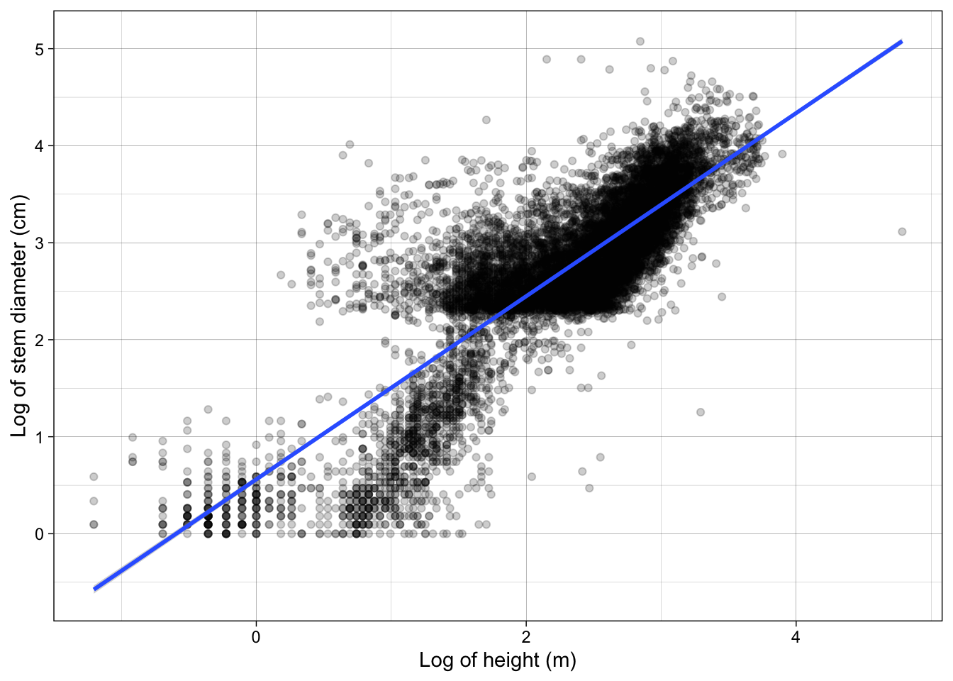
and some text that references all three outputs below:
See @fig-overall-lm, @tbl-overall-glance and @tbl-overall-tidy for results.Using the same approaches we learned above, add a new section called Growth form level analysis and add the code and outputs associated with the growth form level analysis.
Here’s what my section looks like:
## Growth form level analysis
We also fit a model with an interaction term with growth form included.
```{r}
lm_growth <- lm(
log(stem_diameter) ~ log(height) * growth_form,
analysis_df
)
```
```{r}
#| echo: false
#| tbl-cap: "Growth Form interaction model evaluation"
#| label: tbl-growth-glance
library(gt)
lm_growth |> broom::glance() |> gt() |>
fmt_number(decimals = 2)
```
```{r}
#| echo: false
#| tbl-cap: "Growth Form interaction model coefficents"
#| label: tbl-growth-tidy
library(gt)
lm_growth |> broom::tidy() |> gt() |>
fmt_number(decimals = 4) |>
tab_style_body(
columns = "p.value",
style = cell_text(weight = "bold"),
fn = function(x) x < 0.05
)
```
```{r}
#| echo: false
#| fig-cap: "Relationship between stem diameter and height across growth forms."
#| label: fig-growth-formlm
analysis_df %>%
ggplot(aes(x = log(height), y = log(stem_diameter), colour = growth_form)) +
geom_point(alpha = 0.1) +
geom_smooth(method = "lm") +
labs(
x = "Log of height (m)",
y = "Log of stem diameter (cm)",
colour = "Growth forms"
) +
theme_linedraw()
```
See @fig-growth-formlm, @tbl-growth-glance and @tbl-growth-tidy for results.An excellent feature of Quarto with respect to writing scientific reports is the native ability to include citations and references in your document.
The first step to being able to add citations to a Quarto report is to add a bibliography file.
Quarto supports bibliography files in a wide variety of formats including BibLaTeX and CSL.
I’ve included references.bib in data-raw/wood-survey-data-master which contains a number of references in BibTex format:
data-raw/wood-survey-data-master/references.bib
@misc{DP1.10098.001/provisional,
doi = {},
url = {https://data.neonscience.org/data-products/DP1.10098.001},
author = {{National Ecological Observatory Network (NEON)}},
language = {en},
title = {Vegetation structure (DP1.10098.001)},
publisher = {National Ecological Observatory Network (NEON)},
year = {2019}
}
@misc{forestry2012,
organization = {U.S. Forest Service},
title = {Forest Inventory and Analysis National Core Field Guide. Volume I: Field Data
Collection Procedures for Phase 2 Plots},
volume = {1},
pages = {1-472},
year = {2012}
}
@article{Haase,
author = {Haase, Diane},
year = {2008},
month = {01},
pages = {24-30},
title = {Understanding forest seedling quality: measurements and interpretation},
volume = {52},
journal = {Tree Planters' Notes}
}
@article{THORNLEY1999195,
title = {Modelling Stem Height and Diameter Growth in Plants},
journal = {Annals of Botany},
volume = {84},
number = {2},
pages = {195-205},
year = {1999},
issn = {0305-7364},
doi = {https://doi.org/10.1006/anbo.1999.0908},
url = {https://www.sciencedirect.com/science/article/pii/S0305736499909083},
author = {JOHN H.M. THORNLEY},
keywords = {Plant, stem, height, diameter, growth, model, forest, plantation, trees.},
abstract = {A model of stem height and diameter growth in plants is developed. This is formulated and implemented within the framework of an existing tree plantation growth model: the ITE Edinburgh Forest Model. It is proposed that the height:diameter growth rate ratio is a function of a within-plant allocation ratio determined by the transport-resistance model of partitioning, multiplied by a foliage turgor pressure modifier. First it is demonstrated that the method leads to a stable long-term growth trajectory. Diurnal and seasonal dynamics are also examined. Predicted time courses over 20 years of stem mass, stem height, height:diameter ratio, and height:diameter growth rate ratio are presented for six treatments: control, high nitrogen, increased atmospheric carbon dioxide concentration, increased planting density, increased temperature and decreased rainfall. High nitrogen and increased temperature give initially higher stem height:diameter ratios, whereas high CO2gives an initially lower stem height:diameter ratio. However, the responses are complex, reflecting interactions between factors which often have opposing influences on height:diameter ratios, for example: stem density, competition for light and for nitrogen; carbon dioxide and decreased water stress; rainfall, leaching and nitrogen nutrition. The approach relates stem height and diameter growth variables via internal plant variables to environmental and management variables. Potentially, a coherent view of many observations which are sometimes in apparent conflict is provided. These aspects of plant growth can be considered more mechanistically than has hitherto been the case, providing an alternative to the empirical or teleonomic methods which have usually been employed.}
}
@article{CANNELL1984299,
title = {Woody biomass of forest stands},
journal = {Forest Ecology and Management},
volume = {8},
number = {3},
pages = {299-312},
year = {1984},
issn = {0378-1127},
doi = {https://doi.org/10.1016/0378-1127(84)90062-8},
url = {https://www.sciencedirect.com/science/article/pii/0378112784900628},
author = {M.G.R. Cannell},
abstract = {Published data on the total aboveground woody biomass (stems and branches), WT, of 640 forest and woodland stands around the world (Cannell, 1982) were divided into 32 species groups. Differences between groups were examined in the relationship: WT = F(HG) D, where F was a stand form factor; H was mean tree height; G was basal area at breast height; and D was mean wood basic specific gravity. WT was linearly related to (HG); broadleaved species, owing to their greater D, had greater regression coefficients than conifers. Regression coefficients and F factors tended to be smallest in groups having the smallest percentage biomass as branches and greatest in those having most branches. F factors of about 0.5 corresponded to groups having 5–10% branches. The shapes of the woody parts of trees in those groups would conform most closely to quadratic paraboloids as hypothesized by Dawkins (1963) and Gray (1966). But heavily branched broadleaved stands had F factors of 0.6–0.8, and the F factor of tapped Hevea rubber with 81% branches exceeded 1. Thus, for any given G and H, the greatest WT was contained in those forests which had the greatest proportion of branches.}
}To make the reference available to our document to cite, we add the following to our YAML front matter:
bibliography: data-raw/wood-survey-data-master/references.bibwhich should now look a bit like this:
---
title: "Analysis of NEON Woody plant vegetation structure data"
subtitle: "ACCE DTP course"
author: "Anna Krystalli"
date: "2024-03-19"
format:
html:
toc: true
theme: minty
highlight-style: dracula
code-overflow: wrap
df-print: paged
editor: visual
bibliography: data-raw/wood-survey-data-master/references.bib
---We can now use special citation notation to add citations to our document. It is best to do this in the visual editor as available references can be added interactively.
[@THORNLEY1999195; @CANNELL1984299] renders to (THORNLEY 1999; Cannell 1984)
@THORNLEY1999195 renders to THORNLEY (1999)
Quarto will use Pandoc to automatically generate citations and add a bibliography section to the bottom of the document.
Background section with a real citation from the references.bib file.references.bib file.See more details about citations and references.
Your final report should look a bit like:
---
title: "Analysis of NEON Woody plant vegetation structure data"
subtitle: "ACCE DTP course"
author: "Anna Krystalli"
date: "2024-03-19"
format:
html:
toc: true
theme: minty
highlight-style: dracula
df-print: paged
editor: visual
bibliography: data-raw/wood-survey-data-master/references.bib
---
## Background
{width="200"}
The [NEON Woody plant vegetation structure dataset](https://data.neonscience.org/data-products/DP1.10098.001) [@DP1.10098.001/provisional] contains **structure measurements, including height, canopy diameter, and stem diameter, as well as mapped position of individual woody plants across the survey area.**
This data product contains the quality-controlled, native sampling resolution data from in-situ measurements of live and standing dead woody individuals and shrub groups, from all terrestrial NEON sites with qualifying woody vegetation. With some modifications, this protocol adopts guidelines established by the @forestry2012 for measuring tree species. The exact measurements collected per individual depend on growth form, and these measurements are focused on enabling biomass and productivity estimation, estimation of shrub volume and biomass, and calibration / validation of multiple NEON airborne remote-sensing data products.
Our analyses focus on the **relationship between individual stem height and diameter** and how that relationship **varies across growth forms**.
### Data Preparation
Data was prepared for analysis by:
- Compiling all individual raw data files into a single table.
- Merging individual data with plot level data and geolocating individuals.
The data preparation steps are contained in the `data-raw/individuals.R` script.
## Summary statistics
Prepared data were also subset to columns of interest `stem_diameter`, `height` and `growth_form` and rows filtered to complete cases. Liana growth forms were removed.
```{r}
#| label: setup
#| code-fold: true
#| message: false
## Setup ----
# Load libraries
library(dplyr)
library(ggplot2)
# Load data
individual <- readr::read_csv(
here::here("data", "individual.csv")
) %>%
select(stem_diameter, height, growth_form)
## Subset analysis data ----
analysis_df <- individual %>%
filter(complete.cases(.), growth_form != "liana")
## Order growth form levels
gf_levels <- table(analysis_df$growth_form) %>%
sort() %>%
names()
analysis_df <- analysis_df %>%
mutate(growth_form = factor(growth_form,
levels = gf_levels
))
```
The final data set contains a total of **`{r} nrow(analysis_df)`**
```{r}
#| echo: false
#| label: tbl-print
analysis_df
```
```{r}
#| echo: false
#| label: fig-growth-form-counts
#| fig-cap: "Distribution of individual counts across growth forms."
analysis_df %>%
ggplot(aes(
y = growth_form, colour = growth_form,
fill = growth_form
)) +
geom_bar(alpha = 0.5, show.legend = FALSE)
```
@fig-growth-form-counts shows the distribution of individual counts across growth forms in the dataset.
```{r}
#| echo: false
#| label: fig-violin-plots
#| fig-cap: "Distribution of log stem_diameter and log height across growth forms"
analysis_df %>%
tidyr::pivot_longer(
cols = c(stem_diameter, height),
names_to = "var",
values_to = "value"
) %>%
ggplot(aes(
x = log(value), y = growth_form,
colour = growth_form, fill = growth_form
)) +
geom_violin(alpha = 0.5, trim = TRUE, show.legend = FALSE) +
geom_boxplot(alpha = 0.7, show.legend = FALSE) +
facet_grid(~var) +
theme_linedraw()
```
@fig-violin-plots shows the log distribution of stem diameter and log height across growth forms.
# Analysis
## Modelling overall `stem_diameter` as a function of `height`
Initially we fit a linear model of form `log(stem_diameter)` as a function of `log(height)`
```{r}
lm_overall <- lm(
  log(stem_diameter) ~ log(height),
  analysis_df
)
```
```{r}
#| echo: false
#| tbl-cap: "Overall model evaluation"
#| label: tbl-overall-glance
library(gt)
lm_overall |>
  broom::glance() |>
  gt() |>
  fmt_number(decimals = 2)
```
```{r}
#| echo: false
#| tbl-cap: "Overall model coefficents"
#| label: tbl-overall-tidy
library(gt)
lm_overall |> broom::tidy() |>
  gt() |>
  fmt_number(decimals = 4) |>
  tab_style_body(
    columns = "p.value",
    style = cell_text(weight = "bold"),
    fn = function(x) x < 0.05
  )
```
```{r}
#| echo: false
#| fig-cap: "Relationship between stem diameter and height across all data."
#| label: fig-overall-lm
analysis_df %>%
  ggplot(aes(x = log(height), y = log(stem_diameter))) +
  geom_point(alpha = 0.2) +
  geom_smooth(method = "lm") +
  xlab("Log of height (m)") +
  ylab("Log of stem diameter (cm)") +
  theme_linedraw()

```
See @fig-overall-lm, @tbl-overall-glance and @tbl-overall-tidy for results.
## Growth form level analysis

We also fit a model with an interaction term with growth form included.

```{r}
lm_growth <- lm(
  log(stem_diameter) ~ log(height) * growth_form,
  analysis_df
)
```

```{r}
#| echo: false
#| tbl-cap: "Growth Form interaction model evaluation"
#| label: tbl-growth-glance
library(gt)
lm_growth |> broom::glance() |> gt() |>
  fmt_number(decimals = 2)
```

```{r}
#| echo: false
#| tbl-cap: "Growth Form interaction model coefficents"
#| label: tbl-growth-tidy
library(gt)
lm_growth |> broom::tidy() |> gt() |>
  fmt_number(decimals = 4) |>
  tab_style_body(
    columns = "p.value",
    style = cell_text(weight = "bold"),
    fn = function(x) x < 0.05
  )
```


```{r}
#| echo: false
#| fig-cap: "Relationship between stem diameter and height across growth forms."
#| label: fig-growth-formlm
analysis_df %>%
  ggplot(aes(x = log(height), y = log(stem_diameter), colour = growth_form)) +
  geom_point(alpha = 0.1) +
  geom_smooth(method = "lm") +
  labs(
    x = "Log of height (m)",
    y = "Log of stem diameter (cm)",
    colour = "Growth forms"
  ) +
  theme_linedraw()
```

See @fig-growth-formlm, @tbl-growth-glance and @tbl-growth-tidy for results.
## Summary
Our results follow findings in the literature e.g @THORNLEY1999195, @CANNELL1984299 and @Haase.and render to something that looks like this:
To publish to Quarto Pub use the following command in the RStudio Terminal:
Terminal
quarto publish quarto-pub report.qmdFind out more about publishing options.